Profiling MXNet Models
It is often helpful to understand what operations take how much time while running a model. This helps optimize the model to run faster. In this tutorial, we will learn how to profile MXNet models to measure their running time and memory consumption using the MXNet profiler.
The incorrect way to profile
If you have just begun using MXNet, you might be tempted to measure the execution time of your model using Python’s time module like shown below:
from time import time
from mxnet import autograd, nd
import mxnet as mx

start = time()
x = nd.random_uniform(shape=(2000,2000))
y = nd.dot(x, x)
print('Time for matrix multiplication: %f sec\n' % (time() - start))

start = time()
print(y.asnumpy())
print('Time for printing the output: %f sec' % (time() - start))
Time for matrix multiplication: 0.005051 sec
[[501.1584 508.29724 495.65237 ... 492.84705 492.69092 490.0481 ]
[508.81058 507.1822 495.1743 ... 503.10526 497.29315 493.67917]
[489.56598 499.47015 490.17722 ... 490.99945 488.05008 483.28836]
...
[484.0019 495.7179 479.92142 ... 493.69952 478.89194 487.2074 ]
[499.64932 507.65094 497.5938 ... 493.0474 500.74512 495.82712]
[516.0143 519.1715 506.354 ... 510.08878 496.35608 495.42523]]
Time for printing the output: 0.167693 sec
From the output above, it seems as if printing the output takes lot more time that multiplying two large matrices. That doesn’t feel right.
This is because, in MXNet, all operations are executed asynchronously. So, when nd.dot(x, x) returns, the matrix multiplication is not complete, it has only been queued for execution. asnumpy in print(y.asnumpy()) however, waits for the result to be computed and hence takes longer time.
While it is possible to use NDArray.waitall() before and after operations to get running time of operations, it is not a scalable method to measure running time of multiple sets of operations, especially in a Sequential or Hybrid network.
The correct way to profile
The correct way to measure running time of MXNet models is to use MXNet profiler. In the rest of this tutorial, we will learn how to use the MXNet profiler to measure the running time and memory consumption of MXNet models. You can import the profiler and configure it from Python code.
from mxnet import profiler
profiler.set_config(profile_all=True, aggregate_stats=True, filename='profile_output.json')
profile_all enables all types of profiling. You can also individually enable the following types of profiling:
profile_symbolic(boolean): whether to profile symbolic operatorsprofile_imperative(boolean): whether to profile imperative operatorsprofile_memory(boolean): whether to profile memory usageprofile_api(boolean): whether to profile the C API
aggregate_stats aggregates statistics in memory which can then be printed to console by calling profiler.dumps().
Setup: Build a model
Let’s build a small convolutional neural network that we can use for profiling.
from mxnet import gluon
net = gluon.nn.HybridSequential()
with net.name_scope():
    net.add(gluon.nn.Conv2D(channels=20, kernel_size=5, activation='relu'))
    net.add(gluon.nn.MaxPool2D(pool_size=2, strides=2))
    net.add(gluon.nn.Conv2D(channels=50, kernel_size=5, activation='relu'))
    net.add(gluon.nn.MaxPool2D(pool_size=2, strides=2))
    net.add(gluon.nn.Flatten())
    net.add(gluon.nn.Dense(512, activation="relu"))
    net.add(gluon.nn.Dense(10))
We need data that we can run through the network for profiling. We’ll use the MNIST dataset.
from mxnet.gluon.data.vision import transforms
train_data = gluon.data.DataLoader(gluon.data.vision.MNIST(train=True).transform_first(transforms.ToTensor()),
                                   batch_size=64, shuffle=True)
Let’s define a method that will run one training iteration given data and label.
# Use GPU if available
try:
    mx.test_utils.list_gpus(); ctx = mx.gpu()
except:
    ctx = mx.cpu()

# Initialize the parameters with random weights
net.collect_params().initialize(mx.init.Xavier(), ctx=ctx)

# Use SGD optimizer
trainer = gluon.Trainer(net.collect_params(), 'sgd', {'learning_rate': .1})

# Softmax Cross Entropy is a frequently used loss function for multi-classs classification
softmax_cross_entropy = gluon.loss.SoftmaxCrossEntropyLoss()

# A helper function to run one training iteration
def run_training_iteration(data, label):

    # Load data and label is the right context
    data = data.as_in_context(ctx)
    label = label.as_in_context(ctx)

    # Run the forward pass
    with autograd.record():
        output = net(data)
        loss = softmax_cross_entropy(output, label)

    # Run the backward pass
    loss.backward()

    # Apply changes to parameters
    trainer.step(data.shape[0])
Starting and stopping the profiler from Python
When the first forward pass is run on a network, MXNet does a number of housekeeping tasks including inferring the shapes of various parameters, allocating memory for intermediate and final outputs, etc. For these reasons, profiling the first iteration doesn’t provide accurate results. We will, therefore skip the first iteration.
# Run the first iteration without profiling
itr = iter(train_data)
run_training_iteration(*next(itr))
We’ll run the next iteration with the profiler turned on.
data, label = next(itr)

# Ask the profiler to start recording
profiler.set_state('run')

run_training_iteration(*next(itr))

# Ask the profiler to stop recording after operations have completed
mx.nd.waitall()
profiler.set_state('stop')
Between running and stopping the profiler, you can also pause and resume the profiler using profiler.pause() and profiler.resume() respectively to profile only parts of the code you want to profile.
Starting profiler automatically using environment variable
The method described above requires code changes to start and stop the profiler. You can also start the profiler automatically and profile the entire code without any code changes using the MXNET_PROFILER_AUTOSTART environment variable.
MXNet will start the profiler automatically if you run your code with the environment variable MXNET_PROFILER_AUTOSTART set to 1. The profiler output is stored into profile.json in the current directory.
Note that the profiler output could be large depending on your code. It might be helpful to profile only sections of your code using the set_state API described in the previous section.
Increasing granularity of the profiler output
MXNet executes computation graphs in ‘bulk mode’ which reduces kernel launch gaps in between symbolic operators for faster execution. This could reduce the granularity of the profiler output. If you need profiling result of every operator, please set the environment variables MXNET_EXEC_BULK_EXEC_INFERENCE and MXNET_EXEC_BULK_EXEC_TRAIN to 0 to disable the bulk execution mode.
Viewing profiler output
There are two ways to view the information collected by the profiler. You can either view it in the console or you can view a more graphical version in a browser.
1. View in console
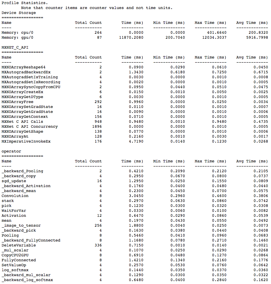
You can use the profiler.dumps() method to view the information collected by the profiler in the console. The collected information contains time taken by each operator, time taken by each C API and memory consumed in both CPU and GPU.
print(profiler.dumps())
2. View in browser
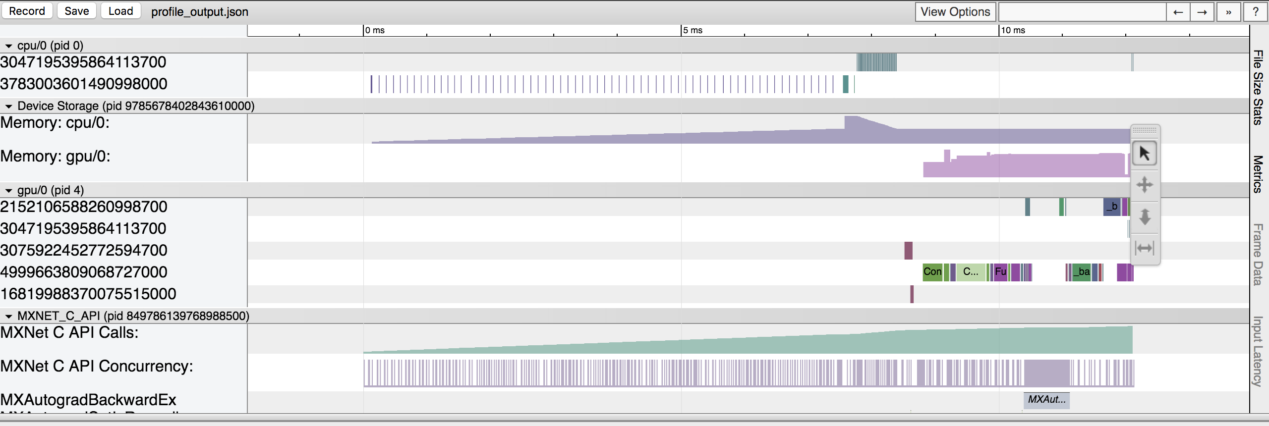
You can also dump the information collected by the profiler into a json file using the profiler.dump() function and view it in a browser.
profiler.dump()
dump() creates a json file which can be viewed using a trace consumer like chrome://tracing in the Chrome browser. Here is a snapshot that shows the output of the profiling we did above.
Let’s zoom in to check the time taken by operators
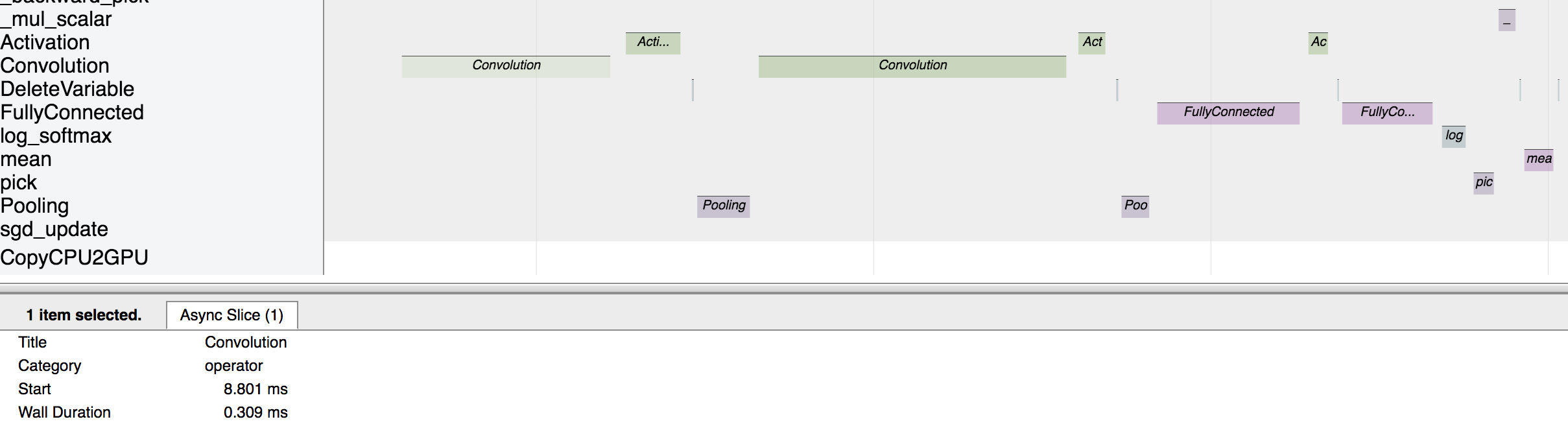
The above picture visualizes the sequence in which the operators were executed and the time taken by each operator.