Image similarity search with InfoGAN
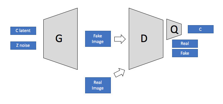
This notebook shows how to implement an InfoGAN based on Gluon. InfoGAN is an extension of GANs, where the generator input is split in 2 parts: random noise and a latent code (see InfoGAN Paper). The codes are made meaningful by maximizing the mutual information between code and generator output. InfoGAN learns a disentangled representation in a completely unsupervised manner. It can be used for many applications such as image similarity search. This notebook uses the DCGAN example from the Straight Dope Book and extends it to create an InfoGAN.
from __future__ import print_function
from datetime import datetime
import logging
import multiprocessing
import os
import sys
import tarfile
import time

import numpy as np
from matplotlib import pyplot as plt
from mxboard import SummaryWriter
import mxnet as mx
from mxnet import gluon
from mxnet import ndarray as nd
from mxnet.gluon import nn, utils
from mxnet import autograd
The latent code vector can contain several variables, which can be categorical and/or continuous. We set n_continuous to 2 and n_categories to 10.
batch_size   = 64
z_dim        = 100
n_continuous = 2
n_categories = 10
ctx = mx.gpu() if mx.context.num_gpus() else mx.cpu()
Some functions to load and normalize images.
lfw_url = 'http://vis-www.cs.umass.edu/lfw/lfw-deepfunneled.tgz'
data_path = 'lfw_dataset'
if not os.path.exists(data_path):
    os.makedirs(data_path)
    data_file = utils.download(lfw_url)
    with tarfile.open(data_file) as tar:
        tar.extractall(path=data_path)
def transform(data, width=64, height=64):
    data = mx.image.imresize(data, width, height)
    data = nd.transpose(data, (2,0,1))
    data = data.astype(np.float32)/127.5 - 1
    if data.shape[0] == 1:
        data = nd.tile(data, (3, 1, 1))
    return data.reshape((1,) + data.shape)
def get_files(data_dir):
    images    = []
    filenames = []
    for path, _, fnames in os.walk(data_dir):
        for fname in fnames:
            if not fname.endswith('.jpg'):
                continue
            img = os.path.join(path, fname)
            img_arr = mx.image.imread(img)
            img_arr = transform(img_arr)
            images.append(img_arr)
            filenames.append(path + "/" + fname)
    return images, filenames
Load the dataset lfw_dataset which contains images of celebrities.
data_dir = 'lfw_dataset'
images, filenames = get_files(data_dir)
split = int(len(images)*0.8)
test_images = images[split:]
test_filenames = filenames[split:]
train_images = images[:split]
train_filenames = filenames[:split]

train_data = gluon.data.ArrayDataset(nd.concatenate(train_images))
train_dataloader = gluon.data.DataLoader(train_data, batch_size=batch_size, shuffle=True, last_batch='rollover', num_workers=multiprocessing.cpu_count()-1)
Generator
Define the Generator model. Architecture is taken from the DCGAN implementation in Straight Dope Book. The Generator consist of 4 layers where each layer involves a strided convolution, batch normalization, and rectified nonlinearity. It takes as input random noise and the latent code and produces an (64,64,3) output image.
class Generator(gluon.HybridBlock):
    def __init__(self, **kwargs):
        super(Generator, self).__init__(**kwargs)
        with self.name_scope():
            self.prev = nn.HybridSequential()
            self.prev.add(nn.Dense(1024, use_bias=False), nn.BatchNorm(), nn.Activation(activation='relu'))
            self.G = nn.HybridSequential()

            self.G.add(nn.Conv2DTranspose(64 * 8, 4, 1, 0, use_bias=False))
            self.G.add(nn.BatchNorm())
            self.G.add(nn.Activation('relu'))
            self.G.add(nn.Conv2DTranspose(64 * 4, 4, 2, 1, use_bias=False))
            self.G.add(nn.BatchNorm())
            self.G.add(nn.Activation('relu'))
            self.G.add(nn.Conv2DTranspose(64 * 2, 4, 2, 1, use_bias=False))
            self.G.add(nn.BatchNorm())
            self.G.add(nn.Activation('relu'))
            self.G.add(nn.Conv2DTranspose(64, 4, 2, 1, use_bias=False))
            self.G.add(nn.BatchNorm())
            self.G.add(nn.Activation('relu'))
            self.G.add(nn.Conv2DTranspose(3, 4, 2, 1, use_bias=False))
            self.G.add(nn.Activation('tanh'))

    def hybrid_forward(self, F, x):
        x = self.prev(x)
        x = F.reshape(x, (0, -1, 1, 1))
        return self.G(x)
Discriminator
Define the Discriminator and Q model. The Q model shares many layers with the Discriminator. Its task is to estimate the code c for a given fake image. It is used to maximize the lower bound to the mutual information.
class Discriminator(gluon.HybridBlock):
    def __init__(self, **kwargs):
        super(Discriminator, self).__init__(**kwargs)
        with self.name_scope():
            self.D = nn.HybridSequential()
            self.D.add(nn.Conv2D(64, 4, 2, 1, use_bias=False))
            self.D.add(nn.LeakyReLU(0.2))
            self.D.add(nn.Conv2D(64 * 2, 4, 2, 1, use_bias=False))
            self.D.add(nn.BatchNorm())
            self.D.add(nn.LeakyReLU(0.2))
            self.D.add(nn.Conv2D(64 * 4, 4, 2, 1, use_bias=False))
            self.D.add(nn.BatchNorm())
            self.D.add(nn.LeakyReLU(0.2))
            self.D.add(nn.Conv2D(64 * 8, 4, 2, 1, use_bias=False))
            self.D.add(nn.BatchNorm())
            self.D.add(nn.LeakyReLU(0.2))

            self.D.add(nn.Dense(1024, use_bias=False), nn.BatchNorm(), nn.Activation(activation='relu'))

            self.prob = nn.Dense(1)
            self.feat = nn.HybridSequential()
            self.feat.add(nn.Dense(128, use_bias=False), nn.BatchNorm(), nn.Activation(activation='relu'))
            self.category_prob = nn.Dense(n_categories)
            self.continuous_mean = nn.Dense(n_continuous)
            self.Q = nn.HybridSequential()
            self.Q.add(self.feat, self.category_prob, self.continuous_mean)

    def hybrid_forward(self, F, x):
        x               = self.D(x)
        prob            = self.prob(x)
        feat            = self.feat(x)
        category_prob   = self.category_prob(feat)
        continuous_mean = self.continuous_mean(feat)

        return prob, category_prob, continuous_mean
The InfoGAN has the following layout.

Discriminator and Generator are the same as in the DCGAN example. On top of the Disciminator is the Q model, which is estimating the code c for given fake images. The Generator’s input is random noise and the latent code c.
Training Loop
Initialize Generator and Discriminator and define correspoing trainer function.
generator = Generator()
generator.hybridize()
generator.initialize(mx.init.Normal(0.002), ctx=ctx)

discriminator = Discriminator()
discriminator.hybridize()
discriminator.initialize(mx.init.Normal(0.002), ctx=ctx)

lr   = 0.0001
beta = 0.5

g_trainer = gluon.Trainer(generator.collect_params(), 'adam', {'learning_rate': lr, 'beta1': beta})
d_trainer = gluon.Trainer(discriminator.collect_params(), 'adam', {'learning_rate': lr, 'beta1': beta})
q_trainer = gluon.Trainer(discriminator.Q.collect_params(), 'adam', {'learning_rate': lr, 'beta1': beta})
Create vectors with real (=1) and fake labels (=0).
real_label = nd.ones((batch_size,), ctx=ctx)
fake_label = nd.zeros((batch_size,),ctx=ctx)
Load a pretrained model.
if os.path.isfile('infogan_d_latest.params') and os.path.isfile('infogan_g_latest.params'):
    discriminator.load_parameters('infogan_d_latest.params', ctx=ctx, allow_missing=True, ignore_extra=True)
    generator.load_parameters('infogan_g_latest.params', ctx=ctx, allow_missing=True, ignore_extra=True)
There are 2 differences between InfoGAN and DCGAN: the extra latent code and the Q network to estimate the code. The latent code is part of the Generator input and it contains mutliple variables (continuous, categorical) that can represent different distributions. In order to make sure that the Generator uses the latent code, mutual information is introduced into the GAN loss term. Mutual information measures how much X is known given Y or vice versa. It is defined as:

The InfoGAN loss is:

where V(D,G) is the GAN loss and the mutual information I(c, G(z, c)) goes in as regularization. The goal is to reach high mutual information, in order to learn meaningful codes for the data.
Define the loss functions. SoftmaxCrossEntropyLoss for the categorical code, L2Loss for the continious code and SigmoidBinaryCrossEntropyLoss for the normal GAN loss.
loss1 = gluon.loss.SigmoidBinaryCrossEntropyLoss()
loss2 = gluon.loss.L2Loss()
loss3 = gluon.loss.SoftmaxCrossEntropyLoss()
This function samples c, z, and concatenates them to create the generator input.
def create_generator_input():

    #create random noise
    z      = nd.random_normal(0, 1, shape=(batch_size, z_dim), ctx=ctx)
    label  = nd.array(np.random.randint(n_categories, size=batch_size)).as_in_context(ctx)
    c1     = nd.one_hot(label, depth=n_categories).as_in_context(ctx)
    c2     = nd.random.uniform(-1, 1, shape=(batch_size, n_continuous)).as_in_context(ctx)

    # concatenate random noise with c which will be the input of the generator
    return nd.concat(z, c1, c2, dim=1), label, c2
Define the training loop.
- The discriminator receives
real_dataandloss1measures how many real images have been identified as real - The discriminator receives
fake_imagefrom the Generator andloss1measures how many fake images have been identified as fake - Update Discriminator. Currently, it is updated every second iteration in order to avoid that the Discriminator becomes too strong. You may want to change that.
- The updated discriminator receives
fake_imageandloss1measures how many fake images have been been identified as real,loss2measures the difference between the sampled continuous latent codecand the output of the Q model andloss3measures the difference between the sampled categorical latent codecand the output of the Q model. - Update Generator and Q
with SummaryWriter(logdir='./logs/') as sw:

    epochs = 1
    counter = 0
    for epoch in range(epochs):
        print("Epoch", epoch)
        starttime = time.time()

        d_error_epoch = nd.zeros((1,), ctx=ctx)
        g_error_epoch = nd.zeros((1,), ctx=ctx)

        for idx, data in enumerate(train_dataloader):

            #get real data and generator input
            real_data = data.as_in_context(ctx)
            g_input, label, c2 = create_generator_input()


            #Update discriminator: Input real data and fake data
            with autograd.record():
                output_real,_,_ = discriminator(real_data)
                d_error_real    = loss1(output_real, real_label)

                # create fake image and input it to discriminator
                fake_image      = generator(g_input)
                output_fake,_,_ = discriminator(fake_image.detach())
                d_error_fake    = loss1(output_fake, fake_label)

                # total discriminator error
                d_error         = d_error_real + d_error_fake

            d_error_epoch += d_error.mean()

            #Update D every second iteration
            if (counter+1) % 2 == 0:
                d_error.backward()
                d_trainer.step(batch_size)

            #Update generator: Input random noise and latent code vector
            with autograd.record():
                fake_image = generator(g_input)
                output_fake, category_prob, continuous_mean = discriminator(fake_image)
                g_error = loss1(output_fake, real_label) + loss3(category_prob, label) + loss2(c2, continuous_mean)

            g_error.backward()
            g_error_epoch += g_error.mean()

            g_trainer.step(batch_size)
            q_trainer.step(batch_size)

            # logging
            if idx % 10 == 0:
                count = idx + 1
                logging.info('speed: {} samples/s'.format(batch_size / (time.time() - starttime)))
                logging.info('discriminator loss = %f, generator loss = %f at iter %d epoch %d'
                         %(d_error_epoch.asscalar()/count,g_error_epoch.asscalar()/count, count, epoch))

                g_input,_,_ = create_generator_input()

                # create some fake image for logging in MXBoard
                fake_image = generator(g_input)

                sw.add_scalar(tag='Loss_D', value={'test':d_error_epoch.asscalar()/count}, global_step=counter)
                sw.add_scalar(tag='Loss_G', value={'test':d_error_epoch.asscalar()/count}, global_step=counter)
                sw.add_image(tag='data_image', image=((fake_image[0]+ 1.0) * 127.5).astype(np.uint8)  , global_step=counter)
                sw.flush()

        discriminator.save_parameters("infogan_d_latest.params")
        generator.save_parameters("infogan_g_latest.params")
Image similarity
Once the InfoGAN is trained, we can use the Discriminator to do an image similarity search. The idea is that the network learned meaningful features from the images based on the mutual information e.g. pose of people in an image.
Load the trained discriminator and retrieve one of its last layers.
discriminator = Discriminator()
discriminator.load_parameters("infogan_d_latest.params", ctx=ctx, ignore_extra=True)

discriminator = discriminator.D[:11]
print (discriminator)

discriminator.hybridize()
Nearest neighbor function, which takes a matrix of features and an input feature vector. It returns the 3 closest features.
def get_knn(features, input_vector, k=3):
    dist = (nd.square(features - input_vector).sum(axis=1))/features.shape[0]
    indices = dist.asnumpy().argsort()[:k]
    return [(index, dist[index].asscalar()) for index in indices]
A helper function to visualize image data.
def visualize(img_array):
    plt.imshow(((img_array.asnumpy().transpose(1, 2, 0) + 1.0) * 127.5).astype(np.uint8))
    plt.axis('off')
Take some images from the test data, obtain its feature vector from discriminator.D[:11] and plot images of the corresponding closest vectors in the feature space.
feature_size = 8192

features = nd.zeros((len(test_images), feature_size), ctx=ctx)

for idx, image in enumerate(test_images):

    feature = discriminator(nd.array(image, ctx=ctx))
    feature = feature.reshape(feature_size,)
    features[idx,:] = feature.copyto(ctx)


for image in test_images[:100]:

    feature = discriminator(mx.nd.array(image, ctx=ctx))
    feature = feature.reshape((feature_size,))
    image   = image.reshape((3,64,64))


    indices = get_knn(features, feature, k=10)
    fig = plt.figure(figsize=(15,12))
    plt.subplot(1,10,1)

    visualize(image)
    for i in range(2,9):
        if indices[i-1][1] < 1.5:
            plt.subplot(1,10,i)
            sim = test_images[indices[i-1][0]].reshape(3,64,64)
            visualize(sim)
    plt.show()
    plt.clf()

How the Generator learns
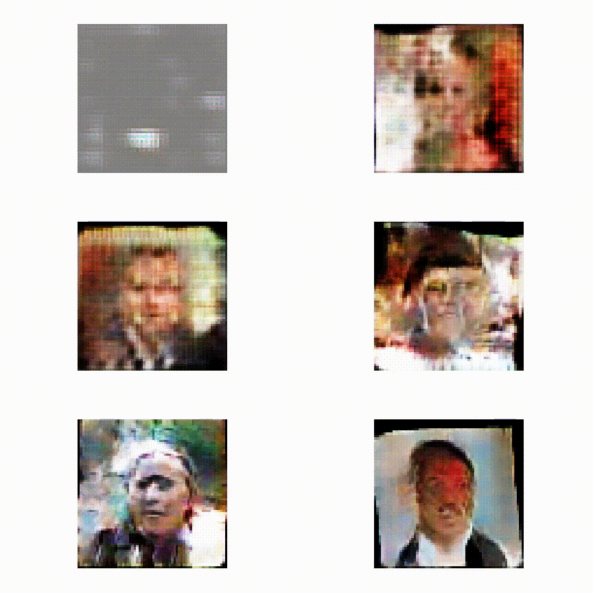
We trained the Generator for a couple of epochs and stored a couple of fake images per epoch. Check the video.

The following function computes the TSNE on the feature matrix and stores the result in a json-file. This file can be loaded with TSNEViewer
import json

from sklearn.manifold import TSNE
from scipy.spatial import distance

tsne = TSNE(n_components=2, learning_rate=150, perplexity=30, verbose=2).fit_transform(features.asnumpy())

# save data to json
data = []
counter = 0
for i,f in enumerate(test_filenames):

    point = [float((tsne[i,k] - np.min(tsne[:,k]))/(np.max(tsne[:,k]) - np.min(tsne[:,k]))) for k in range(2) ]
    data.append({"path": os.path.abspath(os.path.join(os.getcwd(),f)), "point": point})

with open("imagetsne.json", 'w') as outfile:
    json.dump(data, outfile)
Load the file with TSNEViewer. You can now inspect whether similiar looking images are grouped nearby or not.


