Profiling
Profiling
Apache MXNet provides memory profiler which is a way to access what is happening under the hood during runtime. The common scenario is you want to use the profiler for your hybridized model and visualize the outputs via chrome://tracing. Here are the steps you need to do:
- Configure the profiler
set_state('run')before the model is defined- Add
mx.nd.waitall()to enforce synchronization after you have done with some computation (maybe as part of training) - Then add
set_state('stop') - Finally
dumpthe profiling results
Here is a simple example
import mxnet as mx
from mxnet.gluon import nn
from mxnet import profiler

def enable_profiler(profile_filename, run=True, continuous_dump=False, aggregate_stats=False):
    profiler.set_config(profile_symbolic=True,
                        profile_imperative=True,
                        profile_memory=True,
                        profile_api=True,
                        filename=profile_filename,
                        continuous_dump=continuous_dump,
                        aggregate_stats=aggregate_stats)
    if run:
        profiler.set_state('run')

enable_profiler(profile_filename='test_profiler.json', run=True, continuous_dump=True)
profiler.set_state('run')

model = nn.HybridSequential(prefix='net_')
with model.name_scope():
    model.add(nn.Dense(128, activation='tanh'))
    model.add(nn.Dropout(0.5))
    model.add(nn.Dense(64, activation='tanh'),
              nn.Dense(32, in_units=64))
    model.add(nn.Activation('relu'))
model.initialize(ctx=mx.cpu())
model.hybridize()

inputs = mx.sym.var('data')

with mx.autograd.record():
    out = model(mx.nd.zeros((16, 10), ctx=mx.cpu()))
out.backward()
mx.nd.waitall()
profiler.set_state('stop')
profiler.dump(True)
And in chrome://tracing use the load and select test_profiler.json, then you will see something like this
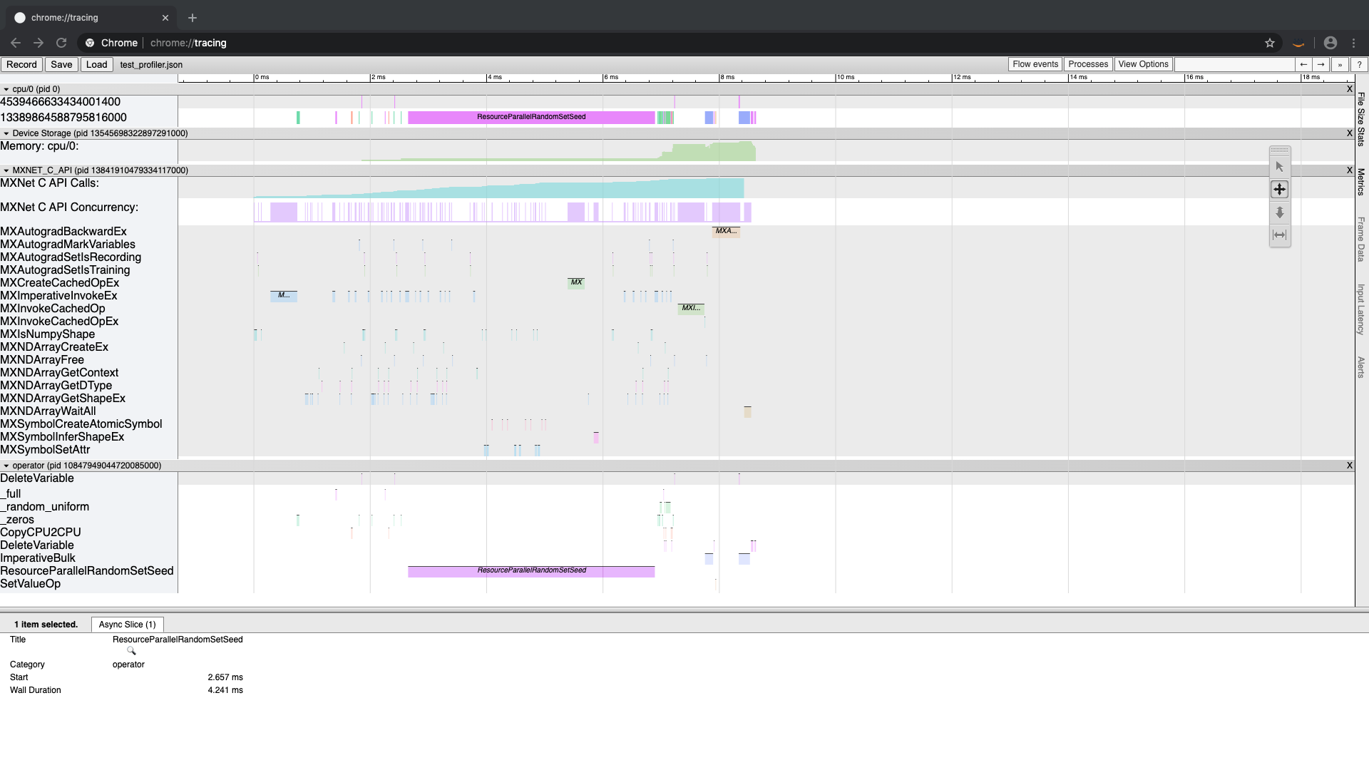 To understand what is going on, we need to dive deep into the MXNet runtime.
Dive deep into MXNet runtime with the profiler
Let's start with a simple example and explain as we go on. The following code creates a 3x3 tensor, computes the diagonal and then sum's along the diagonal (to compute the “trace”). Using the MXNet profiler, we capture internal MXNet behavior and dump it to a string and print it (dumps()) and also dump it to a file (dump()). Then we can import that file in chrome://tracing and view it graphically.
import mxnet as mx
import numpy as np

from mxnet import profiler

#configure the profiler
profiler.set_config(profile_all=True, aggregate_stats=True, filename='trace_profile.json')
#start the profiler collecting data
profiler.set_state('run')

###########################################################
#1. create our data
data = np.linspace(1,9,9).reshape((3,3))

#2. create an MXNet ndarray
a = mx.nd.array(data)

#3. compute on our data and produce results
b = mx.nd.diag(a)
c = mx.nd.sum(b,-1)

#4. wait for computation to finish
mx.nd.waitall()
###########################################################

#stop the profiler
profiler.set_state('stop')

#dump the profiling data as a string
print(profiler.dumps())
#dump the profiling data as a json file that can be viewed graphically
profiler.dump()
When running this code, the dumps function dumps the profiling data to a string and returns it (which we promptly print). This statistical info is shown below.
Profile Statistics:
    Note the difference in units for different entries.
Device Storage
=================
Name                          Total Count    Min Use  (kB)    Max Use  (kB)    Avg Use  (kB)
----                          -----------    -------------    -------------    -------------
Memory: cpu/0                           3          96.0600          96.0760           0.0080

MXNET_C_API
=================
Name                          Total Count        Time (ms)    Min Time (ms)    Max Time (ms)    Avg Time (ms)
----                          -----------        ---------    -------------    -------------    -------------
MXImperativeInvokeEx                    2           0.3360           0.0990           0.2370           0.1680
MXNet C API Calls                      17           0.2320           0.2160           0.2320           0.0080
MXNDArraySyncCopyFromCPU                1           0.1750           0.1750           0.1750           0.1750
MXNDArrayCreateEx                       1           0.1050           0.1050           0.1050           0.1050
MXNDArrayGetShapeEx                    11           0.0210           0.0000           0.0160           0.0019
MXNDArrayWaitAll                        1           0.0200           0.0200           0.0200           0.0200
MXNDArrayGetDType                       1           0.0010           0.0010           0.0010           0.0010
MXNet C API Concurrency                34           0.0000           0.0000           0.0010           0.0000

operator
=================
Name                          Total Count        Time (ms)    Min Time (ms)    Max Time (ms)    Avg Time (ms)
----                          -----------        ---------    -------------    -------------    -------------
sum                                     1           0.0520           0.0520           0.0520           0.0520
diag                                    1           0.0410           0.0410           0.0410           0.0410
WaitForVar                              1           0.0220           0.0220           0.0220           0.0220
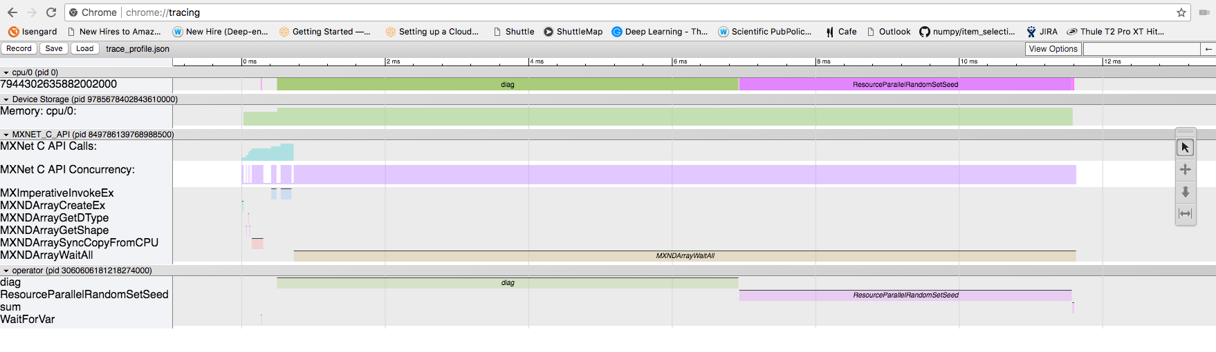
The dump function writes out the same data in a format that can be opened in chrome://tracing and displayed visually. This can be seen in the diagram below.
 The profiling data has captured info about interesting functions that have executed while your program was running. Here are some explanations about what each one does.
The functions in the C_API are:
| Function Name | Description |
|---|---|
| MXImperativeInvokeEx | invokes an operator to perform the computation |
| MXNDArrayCreateEx | creates an ndarray |
| MXNDArrayGetDType | returns the data type of the ndarray |
| MXNDArrayGetShape | returns the shape of the ndarray (as a tuple where each element is the size of a dimension) |
| MXNDArraySyncCopyFromCPU | called when data is initially residing outside of an MXNet data structure (ie. numpy.ndarry rather than mxnet.numpy.ndarray). Data is copied into the MXNet data structure |
| MXNDArrayWaitAll | wait for all asynchronous operations to finish in MXNet. This function is only used in benchmarking to wait for work to happen. In a real program, there is no waiting and data dependencies are evaluated and computation executed as needed in a As Late As Possible (ALAP) way |
The function in the Engine API are:
| Function Name | Description |
|---|---|
| WaitForVar | Takes a variable reference as input and waits until that variable has been computed before returning |
Other API functions:
| Function Name | Description |
|---|---|
| ResourceParallelRandomSetSeed | sets the random number generator seed |
Operators we intended to call in the code:
| Operator Name | Description |
|---|---|
| sum | sum a tensor along a particular axis |
| diag | compute the diagonal of the tensor |
Closer look
From the code, we can identify the major events in our test application
- Initialize our input data
- Creating a new MXNet ndarray using our existing data values
- Compute on our data
- produce the diagonal of the input data
- sum along the diagonal to compute the “trace” of the matrix
- Wait for computation to finish (only needed when profiling)
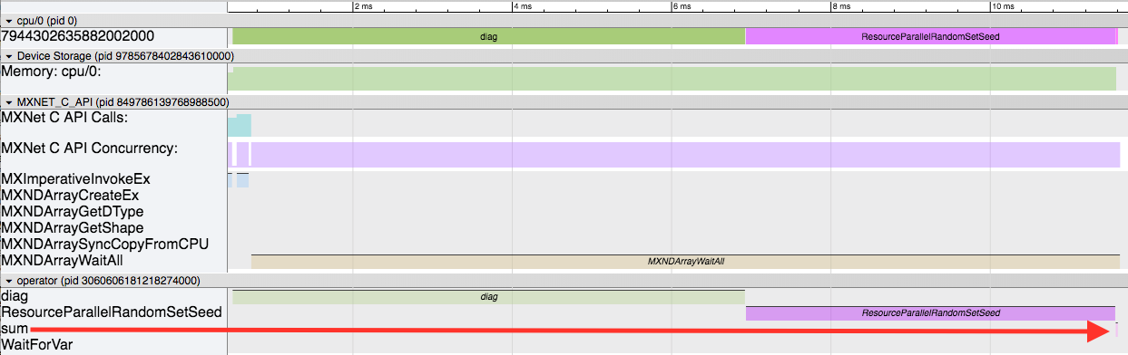
In the following list, #1 uses regular numpy functions to initialize data. MXNet is not involved in this process. In #2, we create an MXNet ndarray and quite a few things happen under the hood. The screenshot below shows a zoomed in portion of the timeline.
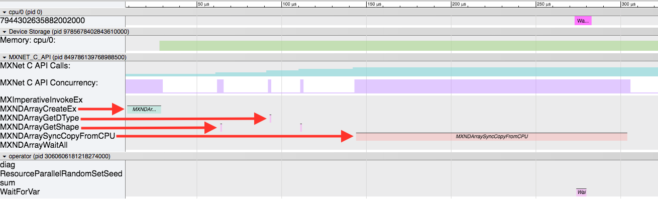 Here, the four red arrows show the important events in this sequence.
- First, the
MXNDArrayCreateExis called to physically allocate space to store the data and other necessary attributes in thendarrayclass. - Then some support functions are called (
MXNDArrayGetShape,MXNDArrayGetDType) while initialing the data structure. - Finally the data is copied from the non-MXNet ndarray into the newly prepared MXNet ndarray by the
MXNDArraySyncCopyFromCPUfunction.
Next, #3 (in our code example) begins the computing process to produce our output data. The screenshot below shows this behavior.
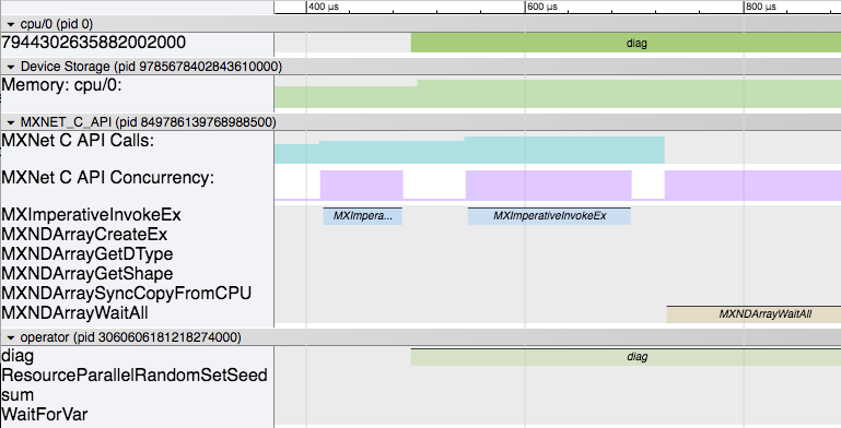 Here you can see that the following sequence of events happen:
MXImperativeInvokeExis called the first time to launch the diagonal operator from #3 (in our code example).- Soon after that the actual
diagoperator begins executing in another thread. - While that is happening, our main thread moves on and calls
MXImperativeInvokeExagain to launch thesumoperator. Just like before, this returns without actually executing the operator and continues. - Lastly, the
MXNDArrayWaitAllis called as the main thread has progressed to #4 in our app. It will wait here while all the computation finishes.
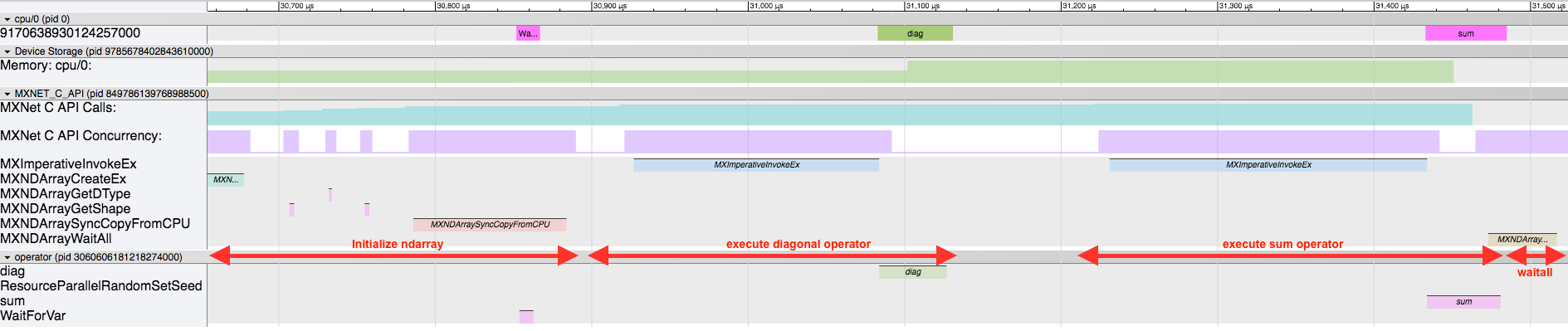
Next lets look at a view of the part of the timeline zoomed to the actual operator execution.
 Here there are 3 main events happening:
- The
diagoperator is executing first. - Then the
ResourceParallelRandomSetSeedruns. - And finally the
sumoperator executes (for a very short time as shown by the big red arrow).
The diag operator running makes sense (although seems to take a little longer than we'd like). At the end, the sum operator runs (very quickly!). But the weird part in the middle is ResourceParallelRandomSetSeed running. This is part of the MXNet resource manager. The resource manager handles temporary space and random number generators needed by the operators. The sum operator requests temporary space in order to compute the sum, and therefore launches the resource manager (for the first time) here. As part of its startup sequence, the random number generator is initialized by setting the seed. So this is some initialization overhead. But let's try and run the app again, running the compute twice, and look at the 2nd run to try and remove this initialization from our profiling.
Here is the modified code:
import mxnet as mx
import numpy as np

from mxnet import profiler

profiler.set_config(profile_all=True, aggregate_stats=True, filename='trace_profile.json')
profiler.set_state('run')

################
# first run
sdata = np.linspace(1,9,9).reshape((3,3))

sa = mx.nd.array(sdata)
sb = mx.nd.diag(sa)
sc = mx.nd.sum(sb,-1)

mx.nd.waitall()
################

################
# second run
data = np.linspace(1,9,9).reshape((3,3))

a = mx.nd.array(data)
b = mx.nd.diag(a)
c = mx.nd.sum(b,-1)

mx.nd.waitall()
################

profiler.set_state('stop')

print(profiler.dumps())
profiler.dump()
Notice that we renamed the variables and made another copy after the waital call. This is so that MXNet doesn’t have to worry about re-using variables, and to segment the 2nd half after the first time initialization.
Here is an overview of the new timeline:
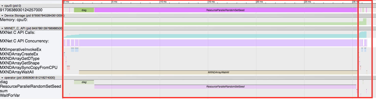 The first red box is the first run, and the 2nd smaller one is the 2nd run. First off, we can see how much smaller the 2nd one is now without any of the initialization routines. Here is a zoomed in view of just the 2nd run.
 We still have the same sequence of events at the beginning to initialize the MXNet ndarray (
MXNDArrayCreateEx, MXNDArrayGetShape, MXNDArrayGetDType, MXNDArraySyncCopyFromCPU). Then the diag operator runs, followed by the sum operator, and finally the waitall. When you look at this, be careful about the assumptions that you make. In this version of the timeline, it appears that the operator executes after the MXImperativeInvokeEx runs, and seems to imply an inherent ordering. But realize that there is no dependency between the diag operator finishing and the next MXImperativeInvokeEx launching the sum operator. In this case, it just-so-happens that the diag operator finishes so quickly that it appears that way. But in reality the main thread is launching the operators and not waiting for them to finish. Lastly, keep in mind that in this case by the time we hit the MXNDArrayWaitAll everything is already done and we return immediately, but in other circumstances it may sit here waiting for everything to finish (like we saw earlier in the first run).