Fine-tuning an ONNX model
Fine-tuning is a common practice in Transfer Learning. One can take advantage of the pre-trained weights of a network, and use them as an initializer for their own task. Indeed, quite often it is difficult to gather a dataset large enough that it would allow training from scratch deep and complex networks such as ResNet152 or VGG16. For example in an image classification task, using a network trained on a large dataset like ImageNet gives a good base from which the weights can be slightly updated, or fine-tuned, to predict accurately the new classes. We will see in this tutorial that this can be achieved even with a relatively small number of new training examples.
Open Neural Network Exchange (ONNX) provides an open source format for AI models. It defines an extensible computation graph model, as well as definitions of built-in operators and standard data types.
In this tutorial we will:
learn how to pick a specific layer from a pre-trained .onnx model file
learn how to load this model in Gluon and fine-tune it on a different dataset
Pre-requisite
To run the tutorial you will need to have installed the following python modules: - MXNet > 1.1.0 - onnx - matplotlib
We recommend that you have first followed this tutorial: - Inference using an ONNX model on MXNet Gluon
import json
import logging
import multiprocessing
import os
import tarfile

logging.basicConfig(level=logging.INFO)

import matplotlib.pyplot as plt
import mxnet as mx
from mxnet import gluon, nd, autograd
from mxnet.gluon.data.vision.datasets import ImageFolderDataset
from mxnet.gluon.data import DataLoader
import mxnet.contrib.onnx as onnx_mxnet
import numpy as np

%matplotlib inline
Downloading supporting files
These are images and a vizualisation script:
image_folder = "images"
utils_file = "utils.py" # contain utils function to plot nice visualization
images = ['wrench.jpg', 'dolphin.jpg', 'lotus.jpg']
base_url = "https://raw.githubusercontent.com/dmlc/web-data/master/mxnet/doc/tutorials/onnx/{}?raw=true"


for image in images:
    mx.test_utils.download(base_url.format("{}/{}".format(image_folder, image)), fname=image,dirname=image_folder)
mx.test_utils.download(base_url.format(utils_file), fname=utils_file)

from utils import *
Downloading a model from the ONNX model zoo
We download a pre-trained model, in our case the GoogleNet model, trained on ImageNet from the ONNX model zoo. The model comes packaged in an archive tar.gz file containing an model.onnx model file.
base_url = "https://s3.amazonaws.com/download.onnx/models/opset_3/"
current_model = "bvlc_googlenet"
model_folder = "model"
archive_file = "{}.tar.gz".format(current_model)
archive_path = os.path.join(model_folder, archive_file)
url = "{}{}".format(base_url, archive_file)
onnx_path = os.path.join(model_folder, current_model, 'model.onnx')

# Download the zipped model
mx.test_utils.download(url, dirname = model_folder)

# Extract the model
if not os.path.isdir(os.path.join(model_folder, current_model)):
    print('Extracting {} in {}...'.format(archive_path, model_folder))
    tar = tarfile.open(archive_path, "r:gz")
    tar.extractall(model_folder)
    tar.close()
    print('Model extracted.')
Downloading the Caltech101 dataset
The Caltech101 dataset is made of pictures of objects belonging to 101 categories. About 40 to 800 images per category. Most categories have about 50 images.
L. Fei-Fei, R. Fergus and P. Perona. Learning generative visual models from few training examples: an incremental Bayesian approach tested on 101 object categories. IEEE. CVPR 2004, Workshop on Generative-Model Based Vision. 2004
data_folder = "data"
dataset_name = "101_ObjectCategories"
archive_file = "{}.tar.gz".format(dataset_name)
archive_path = os.path.join(data_folder, archive_file)
data_url = "https://s3.us-east-2.amazonaws.com/mxnet-public/"

if not os.path.isfile(archive_path):
    mx.test_utils.download("{}{}".format(data_url, archive_file), dirname = data_folder)
    print('Extracting {} in {}...'.format(archive_file, data_folder))
    tar = tarfile.open(archive_path, "r:gz")
    tar.extractall(data_folder)
    tar.close()
    print('Data extracted.')
training_path = os.path.join(data_folder, dataset_name)
testing_path = os.path.join(data_folder, "{}_test".format(dataset_name))
Load the data using an ImageFolderDataset and a DataLoader
We need to transform the images to a format accepted by the network
EDGE = 224
SIZE = (EDGE, EDGE)
BATCH_SIZE = 32
NUM_WORKERS = 6
We transform the dataset images using the following operations: - resize the shorter edge to 224, the longer edge will be greater or equal to 224 - center and crop an area of size (224,224) - transpose the channels to be (3,224,224)
def transform(image, label):
    resized = mx.image.resize_short(image, EDGE)
    cropped, crop_info = mx.image.center_crop(resized, SIZE)
    transposed = nd.transpose(cropped, (2,0,1))
    return transposed, label
The train and test dataset are created automatically by passing the root of each folder. The labels are built using the sub-folders names as label.
train_root
__label1
____image1
____image2
__label2
____image3
____image4
dataset_train = ImageFolderDataset(root=training_path)
dataset_test = ImageFolderDataset(root=testing_path)
We use several worker processes, which means the dataloading and pre-processing is going to be distributed across multiple processes. This will help preventing our GPU from starving and waiting for the data to be copied across
dataloader_train = DataLoader(dataset_train.transform(transform, lazy=False), batch_size=BATCH_SIZE, last_batch='rollover',
                              shuffle=True, num_workers=NUM_WORKERS)
dataloader_test = DataLoader(dataset_test.transform(transform, lazy=False), batch_size=BATCH_SIZE, last_batch='rollover',
                             shuffle=False, num_workers=NUM_WORKERS)
print("Train dataset: {} images, Test dataset: {} images".format(len(dataset_train), len(dataset_test)))
Train dataset: 6996 images, Test dataset: 1681 images
categories = dataset_train.synsets
NUM_CLASSES = len(categories)
BATCH_SIZE = 32
Let’s plot the 1000th image to test the dataset
N = 1000
plt.imshow((transform(dataset_train[N][0], 0)[0].asnumpy().transpose((1,2,0))))
plt.axis('off')
print(categories[dataset_train[N][1]])
Motorbikes
Fine-Tuning the ONNX model
Getting the last layer
Load the ONNX model
sym, arg_params, aux_params = onnx_mxnet.import_model(onnx_path)
This function get the output of a given layer
def get_layer_output(symbol, arg_params, aux_params, layer_name):
    all_layers = symbol.get_internals()
    net = all_layers[layer_name+'_output']
    net = mx.symbol.Flatten(data=net)
    new_args = dict({k:arg_params[k] for k in arg_params if k in net.list_arguments()})
    new_aux = dict({k:aux_params[k] for k in aux_params if k in net.list_arguments()})
    return (net, new_args, new_aux)
Here we print the different layers of the network to make it easier to pick the right one
sym.get_internals()
<Symbol group [data_0, pad0, conv1/7x7_s2_w_0, conv1/7x7_s2_b_0, convolution0, relu0, pad1, pooling0, lrn0, pad2, conv2/3x3_reduce_w_0, conv2/3x3_reduce_b_0, convolution1, relu1, pad3, conv2/3x3_w_0, conv2/3x3_b_0, convolution2, relu2, lrn1, pad4, pooling1, pad5, inception_3a/1x1_w_0, inception_3a/1x1_b_0, convolution3, relu3, pad6, .................................................................................inception_5b/pool_proj_b_0, convolution56, relu56, concat8, pad70, pooling13, dropout0, flatten0, loss3/classifier_w_0, linalg_gemm20, loss3/classifier_b_0, _mulscalar0, broadcast_add0, softmax0]>
We get the network until the output of the flatten0 layer
new_sym, new_arg_params, new_aux_params = get_layer_output(sym, arg_params, aux_params, 'flatten0')
Fine-tuning in gluon
We can now take advantage of the features and pattern detection knowledge that our network learnt training on ImageNet, and apply that to the new Caltech101 dataset.
We pick a context, fine-tuning on CPU will be WAY slower.
ctx = mx.gpu() if mx.context.num_gpus() > 0 else mx.cpu()
We create a symbol block that is going to hold all our pre-trained layers, and assign the weights of the different pre-trained layers to the newly created SymbolBlock
import warnings
with warnings.catch_warnings():
    warnings.simplefilter("ignore")
    pre_trained = gluon.nn.SymbolBlock(outputs=new_sym, inputs=mx.sym.var('data_0'))
net_params = pre_trained.collect_params()
for param in new_arg_params:
    if param in net_params:
        net_params[param]._load_init(new_arg_params[param], ctx=ctx)
for param in new_aux_params:
    if param in net_params:
        net_params[param]._load_init(new_aux_params[param], ctx=ctx)
We create the new dense layer with the right new number of classes (101) and initialize the weights
dense_layer = gluon.nn.Dense(NUM_CLASSES)
dense_layer.initialize(mx.init.Xavier(magnitude=2.24), ctx=ctx)
We add the SymbolBlock and the new dense layer to a HybridSequential network
net = gluon.nn.HybridSequential()
with net.name_scope():
    net.add(pre_trained)
    net.add(dense_layer)
Loss
Softmax cross entropy for multi-class classification
softmax_cross_entropy = gluon.loss.SoftmaxCrossEntropyLoss()
Trainer
Initialize trainer with common training parameters
LEARNING_RATE = 0.0005
WDECAY = 0.00001
MOMENTUM = 0.9
The trainer will retrain and fine-tune the entire network. If we use dense_layer instead of net in the cell below, the gradient updates would only be applied to the new last dense layer. Essentially we would be using the pre-trained network as a featurizer.
trainer = gluon.Trainer(net.collect_params(), 'sgd',
                        {'learning_rate': LEARNING_RATE,
                         'wd':WDECAY,
                         'momentum':MOMENTUM})
Evaluation loop
We measure the accuracy in a non-blocking way, using nd.array to take care of the parallelisation that MXNet and Gluon offers.
def evaluate_accuracy_gluon(data_iterator, net):
   num_instance = 0
   sum_metric = nd.zeros(1,ctx=ctx, dtype=np.int32)
   for i, (data, label) in enumerate(data_iterator):
       data = data.astype(np.float32).as_in_context(ctx)
       label = label.astype(np.int32).as_in_context(ctx)
       output = net(data)
       prediction = nd.argmax(output, axis=1).astype(np.int32)
       num_instance += len(prediction)
       sum_metric += (prediction==label).sum()
   accuracy = (sum_metric.astype(np.float32)/num_instance)
   return accuracy.asscalar()
%%time
print("Untrained network Test Accuracy: {0:.4f}".format(evaluate_accuracy_gluon(dataloader_test, net)))
Untrained network Test Accuracy: 0.0192
Training loop
val_accuracy = 0
for epoch in range(5):
    for i, (data, label) in enumerate(dataloader_train):
        data = data.astype(np.float32).as_in_context(ctx)
        label = label.as_in_context(ctx)

        if i%20==0 and i >0:
            print('Batch [{0}] loss: {1:.4f}'.format(i, loss.mean().asscalar()))

        with autograd.record():
            output = net(data)
            loss = softmax_cross_entropy(output, label)
        loss.backward()
        trainer.step(data.shape[0])

    nd.waitall() # wait at the end of the epoch
    new_val_accuracy = evaluate_accuracy_gluon(dataloader_test, net)
    print("Epoch [{0}] Test Accuracy {1:.4f} ".format(epoch, new_val_accuracy))

    # We perform early-stopping regularization, to prevent the model from overfitting
    if val_accuracy > new_val_accuracy:
        print('Validation accuracy is decreasing, stopping training')
        break
    val_accuracy = new_val_accuracy
Epoch 4, Test Accuracy 0.8942307829856873
Testing
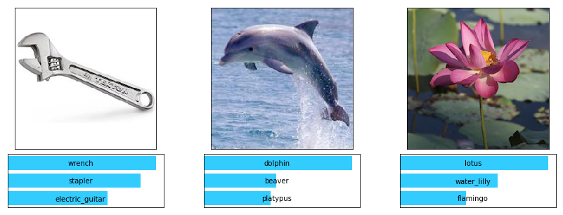
In the previous tutorial, we saw that the network trained on ImageNet couldn’t classify correctly wrench, dolphin, lotus because these are not categories of the ImageNet dataset.
Let’s see if our network fine-tuned on Caltech101 is up for the task:
# Number of predictions to show
TOP_P = 3
# Convert img to format expected by the network
def transform(img):
    return nd.array(np.expand_dims(np.transpose(img, (2,0,1)),axis=0).astype(np.float32), ctx=ctx)
# Load and transform the test images
caltech101_images_test = [plt.imread(os.path.join(image_folder, "{}".format(img))) for img in images]
caltech101_images_transformed = [transform(img) for img in caltech101_images_test]
Helper function to run batches of data
def run_batch(net, data):
    results = []
    for batch in data:
        outputs = net(batch)
        results.extend([o for o in outputs.asnumpy()])
    return np.array(results)
result = run_batch(net, caltech101_images_transformed)
plot_predictions(caltech101_images_test, result, categories, TOP_P)
Great! The network classified these images correctly after being fine-tuned on a dataset that contains images of wrench, dolphin and lotus