Handwritten Digit Recognition
In this tutorial, we’ll give you a step by step walk-through of how to build a hand-written digit classifier using the MNIST dataset.
MNIST is a widely used dataset for the hand-written digit classification task. It consists of 70,000 labeled 28x28 pixel grayscale images of hand-written digits. The dataset is split into 60,000 training images and 10,000 test images. There are 10 classes (one for each of the 10 digits). The task at hand is to train a model using the 60,000 training images and subsequently test its classification accuracy on the 10,000 test images.
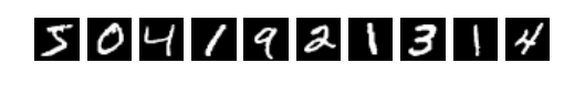
Figure 1: Sample images from the MNIST dataset.
This tutorial uses MXNet’s new high-level interface, gluon package to implement MLP using imperative fashion.
This is based on the Mnist tutorial with symbolic approach. You can find it here.
Prerequisites
To complete this tutorial, we need:
MXNet. See the instructions for your operating system in Setup and Installation.
$ pip install requests jupyter
Loading Data
Before we define the model, let’s first fetch the MNIST dataset.
The following source code downloads and loads the images and the corresponding labels into memory.
import mxnet as mx

# Fixing the random seed
mx.random.seed(42)

mnist = mx.test_utils.get_mnist()
After running the above source code, the entire MNIST dataset should be fully loaded into memory. Note that for large datasets it is not feasible to pre-load the entire dataset first like we did here. What is needed is a mechanism by which we can quickly and efficiently stream data directly from the source. MXNet Data iterators come to the rescue here by providing exactly that. Data iterator is the mechanism by which we feed input data into an MXNet training algorithm and they are very simple to initialize and use and are optimized for speed. During training, we typically process training samples in small batches and over the entire training lifetime will end up processing each training example multiple times. In this tutorial, we’ll configure the data iterator to feed examples in batches of 100. Keep in mind that each example is a 28x28 grayscale image and the corresponding label.
Image batches are commonly represented by a 4-D array with shape (batch_size, num_channels, width, height). For the MNIST dataset, since the images are grayscale, there is only one color channel. Also, the images are 28x28 pixels, and so each image has width and height equal to 28. Therefore, the shape of input is (batch_size, 1, 28, 28). Another important consideration is the order of input samples. When feeding training examples, it is critical that we don’t feed samples with the same
label in succession. Doing so can slow down training. Data iterators take care of this by randomly shuffling the inputs. Note that we only need to shuffle the training data. The order does not matter for test data.
The following source code initializes the data iterators for the MNIST dataset. Note that we initialize two iterators: one for train data and one for test data.
batch_size = 100
train_data = mx.io.NDArrayIter(mnist['train_data'], mnist['train_label'], batch_size, shuffle=True)
val_data = mx.io.NDArrayIter(mnist['test_data'], mnist['test_label'], batch_size)
Approaches
We will cover a couple of approaches for performing the hand written digit recognition task. The first approach makes use of a traditional deep neural network architecture called Multilayer Perceptron (MLP). We’ll discuss its drawbacks and use that as a motivation to introduce a second more advanced approach called Convolution Neural Network (CNN) that has proven to work very well for image classification tasks.
Now, let’s import required nn modules
from __future__ import print_function
import mxnet as mx
from mxnet import gluon
from mxnet.gluon import nn
from mxnet import autograd as ag
Define a network: Multilayer Perceptron
The first approach makes use of a Multilayer Perceptron to solve this problem. We’ll define the MLP using MXNet’s imperative approach.
MLPs consist of several fully connected layers. A fully connected layer or FC layer for short, is one where each neuron in the layer is connected to every neuron in its preceding layer. From a linear algebra perspective, an FC layer applies an affine transform to the n x m input matrix X and outputs a matrix Y of size n x k, where k is the number of neurons in the FC layer. k is also referred to as the hidden size. The output Y is computed according to the equation Y = W X + b. The FC layer has two learnable parameters, the m x k weight matrix W and the m x 1 bias vector b.
In an MLP, the outputs of most FC layers are fed into an activation function, which applies an element-wise non-linearity. This step is critical and it gives neural networks the ability to classify inputs that are not linearly separable. Common choices for activation functions are sigmoid, tanh, and rectified linear unit (ReLU). In this example, we’ll use the ReLU activation function which has several desirable properties and is typically considered a default choice.
The following code declares three fully connected layers with 128, 64 and 10 neurons each. The last fully connected layer often has its hidden size equal to the number of output classes in the dataset. Furthermore, these FC layers uses ReLU activation for performing an element-wise ReLU transformation on the FC layer output.
To do this, we will use Sequential layer type. This is simply a linear stack of neural network layers. nn.Dense layers are nothing but the fully connected layers we discussed above.
# define network
net = nn.Sequential()
with net.name_scope():
    net.add(nn.Dense(128, activation='relu'))
    net.add(nn.Dense(64, activation='relu'))
    net.add(nn.Dense(10))
Initialize parameters and optimizer
The following source code initializes all parameters received from parameter dict using Xavier initializer to train the MLP network we defined above.
For our training, we will make use of the stochastic gradient descent (SGD) optimizer. In particular, we’ll be using mini-batch SGD. Standard SGD processes train data one example at a time. In practice, this is very slow and one can speed up the process by processing examples in small batches. In this case, our batch size will be 100, which is a reasonable choice. Another parameter we select here is the learning rate, which controls the step size the optimizer takes in search of a solution. We’ll pick a learning rate of 0.02, again a reasonable choice. Settings such as batch size and learning rate are what are usually referred to as hyper-parameters. What values we give them can have a great impact on training performance.
We will use Trainer class to apply the SGD optimizer on the initialized parameters.
gpus = mx.test_utils.list_gpus()
ctx =  [mx.gpu()] if gpus else [mx.cpu(0), mx.cpu(1)]
net.initialize(mx.init.Xavier(magnitude=2.24), ctx=ctx)
trainer = gluon.Trainer(net.collect_params(), 'sgd', {'learning_rate': 0.02})
Train the network
Typically, one runs the training until convergence, which means that we have learned a good set of model parameters (weights + biases) from the train data. For the purpose of this tutorial, we’ll run training for 10 epochs and stop. An epoch is one full pass over the entire train data.
We will take following steps for training:
Define Accuracy evaluation metric over training data.
Loop over inputs for every epoch.
Forward input through network to get output.
Compute loss with output and label inside record scope.
Backprop gradient inside record scope.
Update evaluation metric and parameters with gradient descent.
Loss function takes (output, label) pairs and computes a scalar loss for each sample in the mini-batch. The scalars measure how far each output is from the label. There are many predefined loss functions in gluon.loss. Here we use softmax_cross_entropy_loss for digit classification. We will compute loss and do backward propagation inside training scope which is defined by autograd.record().
%%time
epoch = 10
# Use Accuracy as the evaluation metric.
metric = mx.metric.Accuracy()
softmax_cross_entropy_loss = gluon.loss.SoftmaxCrossEntropyLoss()
for i in range(epoch):
    # Reset the train data iterator.
    train_data.reset()
    # Loop over the train data iterator.
    for batch in train_data:
        # Splits train data into multiple slices along batch_axis
        # and copy each slice into a context.
        data = gluon.utils.split_and_load(batch.data[0], ctx_list=ctx, batch_axis=0)
        # Splits train labels into multiple slices along batch_axis
        # and copy each slice into a context.
        label = gluon.utils.split_and_load(batch.label[0], ctx_list=ctx, batch_axis=0)
        outputs = []
        # Inside training scope
        with ag.record():
            for x, y in zip(data, label):
                z = net(x)
                # Computes softmax cross entropy loss.
                loss = softmax_cross_entropy_loss(z, y)
                # Backpropagate the error for one iteration.
                loss.backward()
                outputs.append(z)
        # Updates internal evaluation
        metric.update(label, outputs)
        # Make one step of parameter update. Trainer needs to know the
        # batch size of data to normalize the gradient by 1/batch_size.
        trainer.step(batch.data[0].shape[0])
    # Gets the evaluation result.
    name, acc = metric.get()
    # Reset evaluation result to initial state.
    metric.reset()
    print('training acc at epoch %d: %s=%f'%(i, name, acc))
Prediction
After the above training completes, we can evaluate the trained model by running predictions on validation dataset. Since the dataset also has labels for all test images, we can compute the accuracy metric over validation data as follows:
# Use Accuracy as the evaluation metric.
metric = mx.metric.Accuracy()
# Reset the validation data iterator.
val_data.reset()
# Loop over the validation data iterator.
for batch in val_data:
    # Splits validation data into multiple slices along batch_axis
    # and copy each slice into a context.
    data = gluon.utils.split_and_load(batch.data[0], ctx_list=ctx, batch_axis=0)
    # Splits validation label into multiple slices along batch_axis
    # and copy each slice into a context.
    label = gluon.utils.split_and_load(batch.label[0], ctx_list=ctx, batch_axis=0)
    outputs = []
    for x in data:
        outputs.append(net(x))
    # Updates internal evaluation
    metric.update(label, outputs)
print('validation acc: %s=%f'%metric.get())
assert metric.get()[1] > 0.94
If everything went well, we should see an accuracy value that is around 0.96, which means that we are able to accurately predict the digit in 96% of test images. This is a pretty good result. But as we will see in the next part of this tutorial, we can do a lot better than that.
Convolutional Neural Network
Earlier, we briefly touched on a drawback of MLP when we said we need to discard the input image’s original shape and flatten it as a vector before we can feed it as input to the MLP’s first fully connected layer. Turns out this is an important issue because we don’t take advantage of the fact that pixels in the image have natural spatial correlation along the horizontal and vertical axes. A convolutional neural network (CNN) aims to address this problem by using a more structured weight representation. Instead of flattening the image and doing a simple matrix-matrix multiplication, it employs one or more convolutional layers that each performs a 2-D convolution on the input image.
A single convolution layer consists of one or more filters that each play the role of a feature detector. During training, a CNN learns appropriate representations (parameters) for these filters. Similar to MLP, the output from the convolutional layer is transformed by applying a non-linearity. Besides the convolutional layer, another key aspect of a CNN is the pooling layer. A pooling layer serves to make the CNN translation invariant: a digit remains the same even when it is shifted left/right/up/down by a few pixels. A pooling layer reduces a n x m patch into a single value to make the network less sensitive to the spatial location. Pooling layer is always included after each conv (+ activation) layer in the CNN.
The following source code defines a convolutional neural network architecture called LeNet. LeNet is a popular network known to work well on digit classification tasks. We will use a slightly different version from the original LeNet implementation, replacing the sigmoid activations with tanh activations for the neurons.
A typical way to write your network is creating a new class inherited from gluon.Block class. We can define the network by composing and inheriting Block class as follows:
import mxnet.ndarray as F

class Net(gluon.Block):
    def __init__(self, **kwargs):
        super(Net, self).__init__(**kwargs)
        with self.name_scope():
            # layers created in name_scope will inherit name space
            # from parent layer.
            self.conv1 = nn.Conv2D(20, kernel_size=(5,5))
            self.pool1 = nn.MaxPool2D(pool_size=(2,2), strides = (2,2))
            self.conv2 = nn.Conv2D(50, kernel_size=(5,5))
            self.pool2 = nn.MaxPool2D(pool_size=(2,2), strides = (2,2))
            self.fc1 = nn.Dense(500)
            self.fc2 = nn.Dense(10)

    def forward(self, x):
        x = self.pool1(F.tanh(self.conv1(x)))
        x = self.pool2(F.tanh(self.conv2(x)))
        # 0 means copy over size from corresponding dimension.
        # -1 means infer size from the rest of dimensions.
        x = x.reshape((0, -1))
        x = F.tanh(self.fc1(x))
        x = F.tanh(self.fc2(x))
        return x
We just defined the forward function here, and the backward function to compute gradients is automatically defined for you using autograd. We also imported mxnet.ndarray package to use activation functions from ndarray API.
Now, We will create the network as follows:
net = Net()
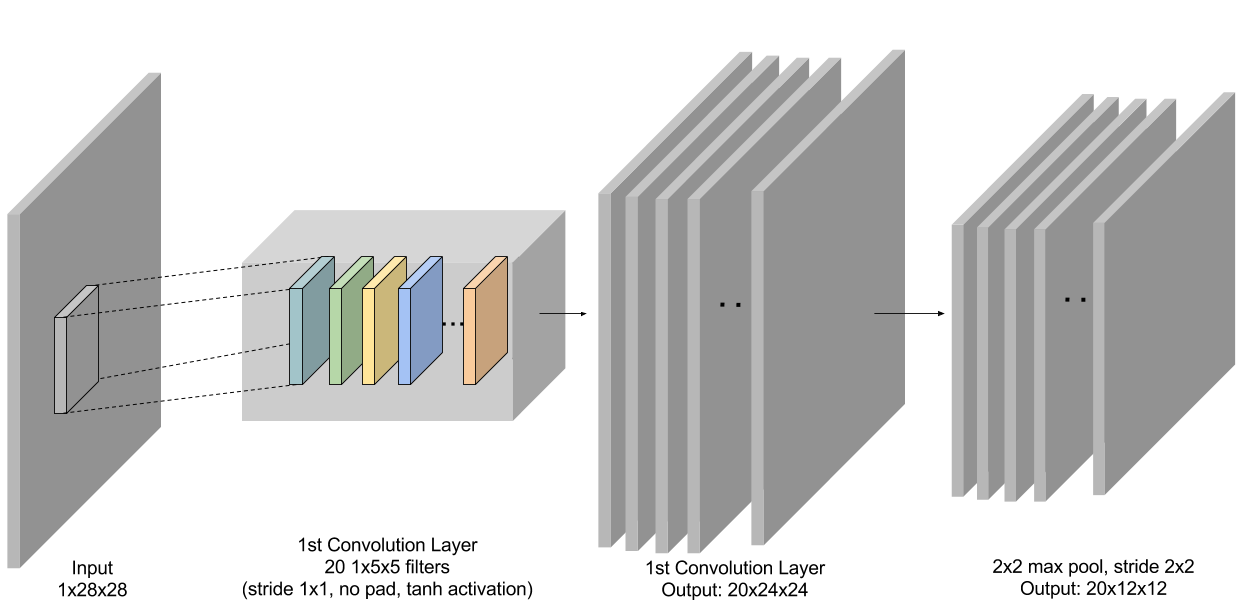
Figure 3: First conv + pooling layer in LeNet.
Now we train LeNet with similar hyper-parameters as before. Note that, if a GPU is available, we recommend using it. This greatly speeds up computation given that LeNet is more complex and compute-intensive than the previous multilayer perceptron. To do so, we only need to change mx.cpu() to mx.gpu() and MXNet takes care of the rest. Just like before, we’ll stop training after 10 epochs.
Training and prediction can be done in the similar way as we did for MLP.
Initialize parameters and optimizer
We will initialize the network parameters as follows:
# set the context on GPU is available otherwise CPU
ctx = [mx.gpu() if mx.test_utils.list_gpus() else mx.cpu()]
net.initialize(mx.init.Xavier(magnitude=2.24), ctx=ctx)
trainer = gluon.Trainer(net.collect_params(), 'sgd', {'learning_rate': 0.03})
Training
# Use Accuracy as the evaluation metric.
metric = mx.metric.Accuracy()
softmax_cross_entropy_loss = gluon.loss.SoftmaxCrossEntropyLoss()

for i in range(epoch):
    # Reset the train data iterator.
    train_data.reset()
    # Loop over the train data iterator.
    for batch in train_data:
        # Splits train data into multiple slices along batch_axis
        # and copy each slice into a context.
        data = gluon.utils.split_and_load(batch.data[0], ctx_list=ctx, batch_axis=0)
        # Splits train labels into multiple slices along batch_axis
        # and copy each slice into a context.
        label = gluon.utils.split_and_load(batch.label[0], ctx_list=ctx, batch_axis=0)
        outputs = []
        # Inside training scope
        with ag.record():
            for x, y in zip(data, label):
                z = net(x)
                # Computes softmax cross entropy loss.
                loss = softmax_cross_entropy_loss(z, y)
                # Backpropogate the error for one iteration.
                loss.backward()
                outputs.append(z)
        # Updates internal evaluation
        metric.update(label, outputs)
        # Make one step of parameter update. Trainer needs to know the
        # batch size of data to normalize the gradient by 1/batch_size.
        trainer.step(batch.data[0].shape[0])
    # Gets the evaluation result.
    name, acc = metric.get()
    # Reset evaluation result to initial state.
    metric.reset()
    print('training acc at epoch %d: %s=%f'%(i, name, acc))
Prediction
Finally, we’ll use the trained LeNet model to generate predictions for the test data.
# Use Accuracy as the evaluation metric.
metric = mx.metric.Accuracy()
# Reset the validation data iterator.
val_data.reset()
# Loop over the validation data iterator.
for batch in val_data:
    # Splits validation data into multiple slices along batch_axis
    # and copy each slice into a context.
    data = gluon.utils.split_and_load(batch.data[0], ctx_list=ctx, batch_axis=0)
    # Splits validation label into multiple slices along batch_axis
    # and copy each slice into a context.
    label = gluon.utils.split_and_load(batch.label[0], ctx_list=ctx, batch_axis=0)
    outputs = []
    for x in data:
        outputs.append(net(x))
    # Updates internal evaluation
    metric.update(label, outputs)
print('validation acc: %s=%f'%metric.get())
assert metric.get()[1] > 0.98
If all went well, we should see a higher accuracy metric for predictions made using LeNet. With CNN we should be able to correctly predict around 98% of all test images.
Summary
In this tutorial, we have learned how to use MXNet to solve a standard computer vision problem: classifying images of hand written digits. You have seen how to quickly and easily build, train and evaluate models such as MLP and CNN with MXNet Gluon package.