Classify Images with a PreTrained Model
Classify Images with a PreTrained Model
MXNet is a flexible and efficient deep learning framework. One of the interesting things that a deep learning algorithm can do is classify real world images.
In this tutorial, we show how to use a pre-trained Inception-BatchNorm network to predict the class of an image. For information about the network architecture, see [1].
The pre-trained Inception-BatchNorm network is able to be downloaded from this link This model gives the recent state-of-art prediction accuracy on image net dataset.
Load the MXNet Package
To get started, load the mxnet package:
require(mxnet)
    ## Loading required package: mxnet
    ## Loading required package: methods
Now load the imager package to load and preprocess the images in R:
require(imager)
    ## Loading required package: imager
    ## Loading required package: plyr
    ## Loading required package: magrittr
    ## Loading required package: stringr
    ## Loading required package: png
    ## Loading required package: jpeg
    ##
    ## Attaching package: 'imager'
    ##
    ## The following object is masked from 'package:magrittr':
    ##
    ##     add
    ##
    ## The following object is masked from 'package:plyr':
    ##
    ##     liply
    ##
    ## The following objects are masked from 'package:stats':
    ##
    ##     convolve, spectrum
    ##
    ## The following object is masked from 'package:graphics':
    ##
    ##     frame
    ##
    ## The following object is masked from 'package:base':
    ##
    ##     save.image
Load the PreTrained Model
Make sure you unzip the pre-trained model in the current folder. Use the model loading function to load the model into R:
model = mx.model.load("Inception/Inception_BN", iteration=39)
Load in the mean image, which is used for preprocessing using:
mean.img = as.array(mx.nd.load("Inception/mean_224.nd")[["mean_img"]])
Load and Preprocess the Image
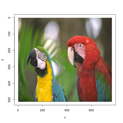
Now, we are ready to classify a real image. In this example, we simply take the parrots image from the imager package. You can use another image, if you prefer.
Load and plot the image:
    im <- load.image(system.file("extdata/parrots.png", package="imager"))
    plot(im)

Before feeding the image to the deep network, we need to perform some preprocessing to make the image meet the deep network input requirements. Preprocessing includes cropping and subtracting the mean. Because MXNet is deeply integrated with R, we can do all the processing in an R function:
    preproc.image <- function(im, mean.image) {
      # crop the image
      shape <- dim(im)
      short.edge <- min(shape[1:2])
      xx <- floor((shape[1] - short.edge) / 2)
      yy <- floor((shape[2] - short.edge) / 2)
      cropped <- crop.borders(im, xx, yy)
      # resize to 224 x 224, needed by input of the model.
      resized <- resize(cropped, 224, 224)
      # convert to array (x, y, channel)
      arr <- as.array(resized) * 255
      dim(arr) <- c(224, 224, 3)
      # subtract the mean
      normed <- arr - mean.img
      # Reshape to format needed by mxnet (width, height, channel, num)
      dim(normed) <- c(224, 224, 3, 1)
      return(normed)
    }
Use the defined preprocessing function to get the normalized image:
normed <- preproc.image(im, mean.img)
Classify the Image
Now we are ready to classify the image! Use the predict function
to get the probability over classes:
    prob <- predict(model, X=normed)
    dim(prob)
## [1] 1000 1
As you can see, prob is a 1 times 1000 array, which gives the probability
over the 1000 image classes of the input.
Use the max.col on the transpose of prob to get the class index:
    max.idx <- max.col(t(prob))
    max.idx
## [1] 89
The index doesn't make much sense, so let's see what it really means. Read the names of the classes from the following file:
synsets <- readLines("Inception/synset.txt")
Let's see what the image really is:
print(paste0("Predicted Top-class: ", synsets [[max.idx]]))
## [1] "Predicted Top-class: n01818515 macaw"
It's a macaw!
Reference
[1] Ioffe, Sergey, and Christian Szegedy. "Batch normalization: Accelerating deep network training by reducing internal covariate shift." arXiv preprint arXiv:1502.03167 (2015).

 R Guide
  R
Tutorials
  R API Reference