Sparse NDArrays with Gluon
When working on machine learning problems, you may encounter situations where the input data is sparse (i.e. the majority of values are zero). One example of this is in recommendation systems. You could have millions of user and product features, but only a few of these features are present for each sample. Without special treatment, the sheer magnitude of the feature space can lead to out-of-memory situations and cause significant slowdowns when training and making predictions.
MXNet supports a number of sparse storage types (often called stype for short) for these situations. In this tutorial, we’ll start by generating some sparse data, write it to disk in the LibSVM format and then read back using the LibSVMIter for training. We use the Gluon API to train the model and leverage sparse storage types such as
CSRNDArray and RowSparseNDArray to maximise performance and memory efficiency.
import mxnet as mx
import numpy as np
import time
Generating Sparse Data
You will most likely have a sparse dataset in mind already if you’re reading this tutorial, but let’s create a dummy dataset to use in the examples that follow. Using rand_ndarray we will generate 1000 samples, each with 1,000,000 features of which 99.999% of values will be zero (i.e. 10 non-zero features for each sample). We take this as our input data for training and calculate a label based on an arbitrary rule: whether the feature sum is higher than average.
num_samples = 1000
num_features = 1000000
data = mx.test_utils.rand_ndarray((num_samples, num_features), stype='csr', density=0.00001)
# generate label: 1 if row sum above average, 0 otherwise.
label = data.sum(axis=1) > data.sum(axis=1).mean()
print(type(data))
print(data[:10].asnumpy())
print('{:,.0f} elements'.format(np.product(data.shape)))
print('{:,.0f} non-zero elements'.format(data.data.size))
<class 'mxnet.ndarray.sparse.CSRNDArray'>
[[0. 0. 0. ... 0. 0. 0.]
 [0. 0. 0. ... 0. 0. 0.]
 [0. 0. 0. ... 0. 0. 0.]
 ...
 [0. 0. 0. ... 0. 0. 0.]
 [0. 0. 0. ... 0. 0. 0.]
 [0. 0. 0. ... 0. 0. 0.]]
1,000,000,000 elements
10,000 non-zero elements
Our storage type is CSR (Compressed Sparse Row) which is the ideal type for sparse data along multiple axes. See this in-depth tutorial for more information. Just to confirm the generation process ran correctly, we can see that the vast majority of values are indeed zero. One of the first questions to ask would be how much memory is saved by storing this data in a
CSRNDArray versus a standard NDArray. Since sparse arrays are constructed from many components (e.g. data, indices and indptr) we define a function called get_nbytes to calculate the number of bytes taken in memory to store an array. We compare the same data stored in a standard
NDArray (with data.tostype('default')) to the CSRNDArray.
def get_nbytes(array):
    fn = lambda a: a.size * np.dtype(a).itemsize
    if isinstance(array, mx.ndarray.sparse.CSRNDArray):
        return fn(array.data) + fn(array.indices) + fn(array.indptr)
    elif isinstance(array, mx.ndarray.sparse.RowSparseNDArray):
        return fn(array.data) + fn(array.indices)
    elif isinstance(array, mx.ndarray.NDArray):
        return fn(array)
    else:
        TypeError('{} not supported'.format(type(array)))
print('NDarray:', get_nbytes(data.tostype('default'))/1000000, 'MBs')
print('CSRNDArray', get_nbytes(data)/1000000, 'MBs')
NDarray: 4000.0 MBs
CSRNDArray 0.128008 MBs
Given the extremely high sparsity of the data, we observe a huge memory saving here! 0.13 MBs versus 4 GBs: ~30,000 times smaller. You can experiment with the amount of sparsity and see how these two storage types compare. When the number of non-zero values increases, this difference will reduce. And when the number of non-zero values exceeds ~1/3 you will find that this sparse storage type take more memory than dense! So use wisely.
Writing Sparse Data
Since there is such a large size difference between dense and sparse storage formats here, we ideally want to store the data on disk in a sparse storage format too. MXNet supports a format called LibSVM and has a data iterator called LibSVMIter specifically for data formatted this way.
A LibSVM file has a row for each sample, and each row starts with the label: in this case 0.0 or 1.0 since we have a classification task. After this we have a variable number of key:value pairs separated by spaces, where the key is column/feature index and the value is the value of that feature. When working with your own sparse data in a custom format you should try to convert your data into this format. We define a save_as_libsvm function to save the data
(CSRNDArray) and label (NDArray) to disk in LibSVM format.
def save_as_libsvm(filepath, data, label):
    with open(filepath, 'w') as openfile:
        for row_idx in range(data.shape[0]):
            data_sample = data[row_idx]
            label_sample = label[row_idx]
            col_idxs = data_sample.indices.asnumpy().tolist()
            values = data_sample.data.asnumpy().tolist()
            label_str = str(label_sample.asscalar())
            value_strs = ['{}:{}'.format(idx, value) for idx, value in zip(col_idxs, values)]
            value_str = " ".join(value_strs)
            sample_str = '{} {}\n'.format(label_str, value_str)
            openfile.write(sample_str)
filepath = 'dataset.libsvm'
save_as_libsvm(filepath, data, label)
We have now written the data and label to disk, and can inspect the first 10 lines of the file:
with open(filepath, 'r') as openfile:
    lines = [openfile.readline() for _ in range(10)]
for line in lines:
    print(line[:80] + '...' if len(line) > 80 else line)
0.0 35454:0.22486156225204468 80954:0.39130592346191406 81941:0.1988530308008194...
1.0 37029:0.5980494618415833 52916:0.15797750651836395 71623:0.32251599431037903...
1.0 89962:0.47770974040031433 216426:0.21326342225074768 271027:0.18589609861373...
1.0 7071:0.9432336688041687 81664:0.7788773775100708 117459:0.8166475296020508 4...
0.0 380966:0.16906292736530304 394363:0.7987179756164551 458442:0.56873309612274...
0.0 89361:0.9099966287612915 141813:0.5927085280418396 282489:0.293381005525589 ...
0.0 150427:0.4747847020626068 169376:0.2603490948677063 179377:0.237988427281379...
0.0 49774:0.2822582423686981 91245:0.5794865489006042 102970:0.7004560232162476 ...
1.0 97133:0.0024336236529052258 109855:0.9895315766334534 116765:0.2465638816356...
0.0 803440:0.4020800292491913
Some storage overhead is introduced by serializing the data as characters (with spaces and colons). dataset.libsvm is 250 KBs but the original data and label were 132 KBs combined. Compared with the 4GB dense NDArray though, this isn’t a huge issue.
Reading Sparse Data
Using LibSVMIter, we can quickly and easily load data into batches ready for training. Although Gluon Datasets can be written to return sparse arrays, Gluon DataLoaders currently convert each sample to dense before stacking up to create the batch. As a result, LibSVMIter is the recommended method of loading sparse data in batches.
Similar to using a DataLoader, you must specify the required batch_size. Since we’re dealing with sparse data and the column shape isn’t explicitly stored in the LibSVM file, we additionally need to provide the shape of the data and label. Our LibSVMIter returns batches in a slightly different form to a
DataLoader. We get DataBatch objects instead of tuple.
data_iter = mx.io.LibSVMIter(data_libsvm=filepath, data_shape=(num_features,), label_shape=(1,), batch_size=10)
for batch in data_iter:
    data = batch.data[0]
    print('data.stype: {}'.format(data.stype))
    label = batch.label[0]
    print('label.stype: {}'.format(label.stype))
    break
data.stype: csr
label.stype: default
We can see that data and label are in the appropriate storage formats, given their sparse and dense values respectively. We can avoid out-of-memory issues that might have occurred if data was in dense storage format. Another benefit of storing the data efficiently is the reduced data transfer time when using GPUs. Although the transfer time for a single batch is small, we transfer data and label to the GPU every iteration so this time can become significant. We will time the
transfer of the sparse data to GPU (if available) and compare to the time for its dense counterpart.
ctx = mx.gpu() if mx.test_utils.list_gpus() else mx.cpu()
%%timeit
data_on_ctx = data.as_in_context(ctx)
data_on_ctx.wait_to_read()
192 microseconds +- 51.1 microseconds per loop (mean +- std. dev. of 7 runs, 1 loop each)
print('sparse batch: {} MBs'.format(get_nbytes(data)/1000000))
data = data.tostype('default')  # avoid timing this sparse to dense conversion
print('dense batch: {} MBs'.format(get_nbytes(data)/1000000))
sparse batch: 0.001348 MBs
dense batch: 40.0 MBs
%%timeit
data_on_ctx = data.as_in_context(ctx)
data_on_ctx.wait_to_read()
4 ms +- 36.8 microseconds per loop (mean +- std. dev. of 7 runs, 100 loops each)
Although results will change depending on system specifications and degree of sparsity, the sparse array can be transferred from CPU to GPU significantly faster than the dense array. We see a ~25x speed up for sparse vs dense for this specific batch of data.
Gluon Models for Sparse Data
Our next step is to define a network. We have an input of 1,000,000 features and we want to make a binary prediction. We don’t have any spatial or temporal relationships between features, so we’ll use a 3 layer fully-connected network where the last layer has 1 output unit (with sigmoid activation). Since we’re working with sparse data, we’d ideally like to use network operators that can exploit this sparsity for improved performance and memory efficiency.
Gluon’s nn.Dense block can used with CSRNDArray input arrays but it doesn’t exploit the sparsity. Under the hood, Dense uses the FullyConnected operator which isn’t optimized for
CSRNDArray arrays. We’ll implement a Block that does exploit this sparsity, but first, let’s just remind ourselves of the Dense implementation by creating an equivalent Block called FullyConnected.
class FullyConnected(mx.gluon.HybridBlock):
    def __init__(self, in_units, units):
        super(FullyConnected, self).__init__()
        with self.name_scope():
            self._units = units
            self.weight = self.params.get('weight', shape=(units, in_units),
                                          init=None, allow_deferred_init=True,
                                          dtype='float32', stype='default', grad_stype='default')
            self.bias = self.params.get('bias', shape=(units),
                                          init='zeros', allow_deferred_init=True,
                                          dtype='float32', stype='default', grad_stype='default')

    def hybrid_forward(self, F, x, weight, bias):
        return F.FullyConnected(x, weight, bias, num_hidden=self._units)
Our weight and bias parameters are dense (see stype='default') and so are their gradients (see grad_stype='default'). Our weight parameter has shape (units, in_units) because the FullyConnected operator performs the following calculation:
We could instead have created our parameter with shape (in_units, units) and avoid the transpose of the weight matrix. We’ll see why this is so important later on. And instead of FullyConnected we could have used mx.sparse.dot to fully exploit the sparsity of the
CSRNDArray input arrays. We’ll now implement an alternative Block called FullyConnectedSparse using these ideas. We take grad_stype of the weight as an argument (called weight_grad_stype), since we’re going to change this later on.
class FullyConnectedSparse(mx.gluon.HybridBlock):
    def __init__(self, in_units, units, weight_grad_stype='default'):
        super(FullyConnectedSparse, self).__init__()
        with self.name_scope():
            self._units = units
            self.weight = self.params.get('weight', shape=(in_units, units),
                                          init=None, allow_deferred_init=True,
                                          dtype='float32', stype='default', grad_stype=weight_grad_stype)
            self.bias = self.params.get('bias', shape=(units),
                                          init='zeros', allow_deferred_init=True,
                                          dtype='float32', stype='default', grad_stype='default')

    def hybrid_forward(self, F, x, weight, bias):
        return F.sparse.dot(x, weight) + bias
Once again, we’re using a dense weight, so both FullyConnected and FullyConnectedSparse will return dense array outputs. When constructing a multi-layer network therefore, only the first layer needs to be optimized for sparse inputs. Our first layer is often responsible for reducing the feature dimension dramatically (e.g. 1,000,000 features down to 128 features). We’ll set the number of units in our 3 layers to be 128, 8 and 1.
We will use timeit to check the performance of these two variants, and analyse some MXNet Profiler traces that have been created from these benchmarks. Additionally, we will inspect the memory usage of the weights (and gradients) using the print_memory_allocation function defined below:
def print_memory_allocation(net, block_idxs):
    blocks = [net[block_idx] for block_idx in block_idxs]
    weight_nbytes = [get_nbytes(b.weight.data()) for b in blocks]
    weight_nbytes_pct = [b/sum(weight_nbytes) for b in weight_nbytes]
    weight_grad_nbytes = [get_nbytes(b.weight.grad()) for b in blocks]
    weight_grad_nbytes_pct = [b/sum(weight_grad_nbytes) for b in weight_grad_nbytes]
    print("Memory Allocation for Weight:")
    for i in range(len(block_idxs)):
        print('{:7.3f} MBs ({:7.3f}%) for {:<40}'.format(weight_nbytes[i]/1000000,
                                                              weight_nbytes_pct[i]*100,
                                                              blocks[i].name))
    print("Memory Allocation for Weight Gradient:")
    for i in range(len(block_idxs)):
        print('{:7.3f} MBs ({:7.3f}%) for {:<40}'.format(weight_grad_nbytes[i]/1000000,
                                                              weight_grad_nbytes_pct[i]*100,
                                                              blocks[i].name))
Benchmark: FullyConnected
We’ll create a network using nn.Dense and benchmark the training.
net = mx.gluon.nn.Sequential()
net.add(
    mx.gluon.nn.Dense(in_units=num_features, units=128),
    mx.gluon.nn.Activation('sigmoid'),
    mx.gluon.nn.Dense(in_units=128, units=8),
    mx.gluon.nn.Activation('sigmoid'),
    mx.gluon.nn.Dense(in_units=8, units=1),
    mx.gluon.nn.Activation('sigmoid'),
)
net.initialize(ctx=ctx)
trainer = mx.gluon.Trainer(net.collect_params(), 'sgd')
loss_fn = mx.gluon.loss.SigmoidBinaryCrossEntropyLoss()
%%timeit
data_iter.reset()
for batch in data_iter:
    data = batch.data[0]
    data = data.as_in_context(ctx)
    label = batch.label[0].as_in_context(ctx)
    with mx.autograd.record():
        pred = net(data)
        loss = loss_fn(pred, label)
    loss.backward()
    trainer.step(data.shape[0])
    loss.wait_to_read()
532 ms +- 3.47 ms per loop (mean +- std. dev. of 7 runs, 1 loop each)
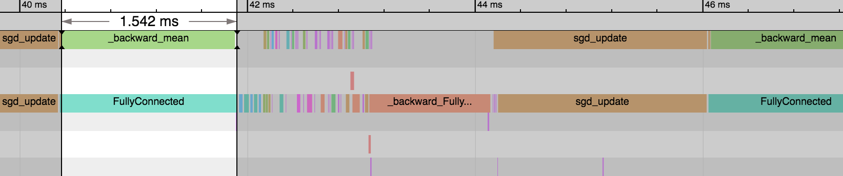
We can see the first FullyConnected operator takes a significant proportion of time to execute (~25% of the iteration) because there are 1,000,000 input features (to 128). After this, the other FullyConnected operators are much faster because they have input features of 128 (to 8) and 8 (to 1). On the backward pass, we see the same pattern (but
in reverse). And finally, the parameter update step takes a large amount of time on the weight matrix of the first FullyConnected Block. When checking the memory allocations below, we can see the weight matrix of the first FullyConnected Block is responsible for 99.999% of the memory compared to other FullyConnected weight matrices.
print_memory_allocation(net, block_idxs=[0, 2, 4])
Memory Allocation for Weight:
512.000 MBs ( 99.999%) for dense0
  0.004 MBs (  0.001%) for dense1
  0.000 MBs (  0.000%) for dense2
Memory Allocation for Weight Gradient:
512.000 MBs ( 99.999%) for dense0
  0.004 MBs (  0.001%) for dense1
  0.000 MBs (  0.000%) for dense2
Benchmark: FullyConnectedSparse
We will now switch the first layer from FullyConnected to FullyConnectedSparse.
net = mx.gluon.nn.Sequential()
net.add(
    FullyConnectedSparse(in_units=num_features, units=128),
    mx.gluon.nn.Activation('sigmoid'),
    FullyConnected(in_units=128, units=8),
    mx.gluon.nn.Activation('sigmoid'),
    FullyConnected(in_units=8, units=1),
    mx.gluon.nn.Activation('sigmoid'),
)
net.initialize(ctx=ctx)
trainer = mx.gluon.Trainer(net.collect_params(), 'sgd')
loss_fn = mx.gluon.loss.SigmoidBinaryCrossEntropyLoss()
%%timeit
data_iter.reset()
for batch in data_iter:
    data = batch.data[0]
    data = data.as_in_context(ctx)
    label = batch.label[0].as_in_context(ctx)
    with mx.autograd.record():
        pred = net(data)
        loss = loss_fn(pred, label)
    loss.backward()
    trainer.step(data.shape[0])
    loss.wait_to_read()
528 ms +- 22.7 ms per loop (mean +- std. dev. of 7 runs, 1 loop each)
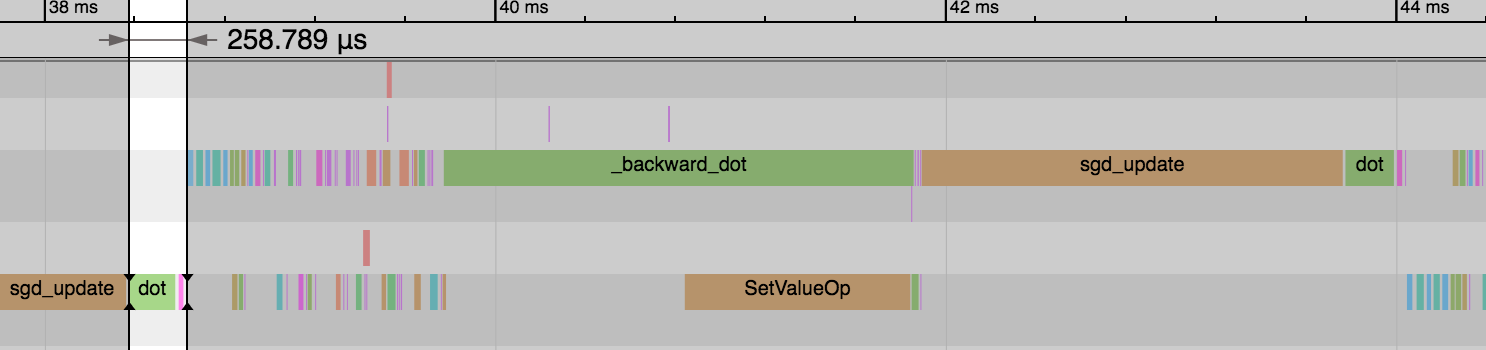
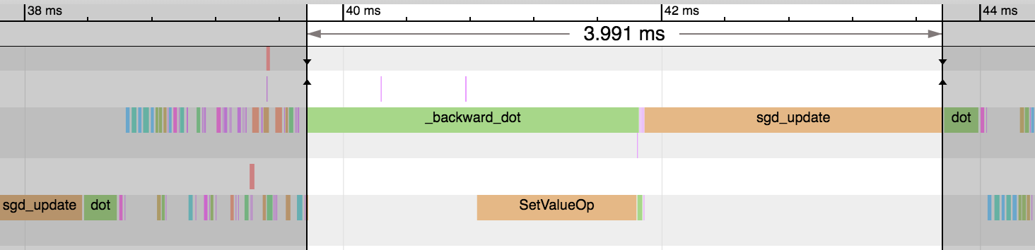
We see the forward pass of dot and add (equivalent to FullyConnected operator) is much faster now: 1.54ms vs 0.26ms. And this explains the reduction in overall time for the epoch. We didn’t gain any benefit on the backward pass or parameter updates though.
Our first weight matrix and its gradients still take up the same amount of memory as before.
print_memory_allocation(net, block_idxs=[0, 2, 4])
Memory Allocation for Weight:
512.000 MBs ( 99.999%) for fullyconnectedsparse0
  0.004 MBs (  0.001%) for fullyconnected0
  0.000 MBs (  0.000%) for fullyconnected1
Memory Allocation for Weight Gradient:
512.000 MBs ( 99.999%) for fullyconnectedsparse0
  0.004 MBs (  0.001%) for fullyconnected0
  0.000 MBs (  0.000%) for fullyconnected1
Benchmark: FullyConnectedSparse with grad_stype=row_sparse
One useful outcome of sparsity in our CSRNDArray input is that our gradients will be row sparse. We can exploit this fact to give us potentially huge memory savings and speed improvements. Creating our weight parameter with shape (units, in_units) and not transposing in the forward pass are important pre-requisite for obtaining row sparse gradients. Using
nn.Dense would have led to column sparse gradients which are not supported in MXNet. We previously had grad_stype of the weight parameter in the first layer set to 'default' so we were handling the gradient as a dense array. Switching this to 'row_sparse' can give us these potential improvements.
net = mx.gluon.nn.Sequential()
net.add(
    FullyConnectedSparse(in_units=num_features, units=128, weight_grad_stype='row_sparse'),
    mx.gluon.nn.Activation('sigmoid'),
    FullyConnected(in_units=128, units=8),
    mx.gluon.nn.Activation('sigmoid'),
    FullyConnected(in_units=8, units=1),
    mx.gluon.nn.Activation('sigmoid'),
)
net.initialize(ctx=ctx)
trainer = mx.gluon.Trainer(net.collect_params(), 'sgd')
loss_fn = mx.gluon.loss.SigmoidBinaryCrossEntropyLoss()
%%timeit
data_iter.reset()
for batch in data_iter:
    data = batch.data[0]
    data = data.as_in_context(ctx)
    label = batch.label[0].as_in_context(ctx)
    with mx.autograd.record():
        pred = net(data)
        loss = loss_fn(pred, label)
    loss.backward()
    trainer.step(data.shape[0])
    loss.wait_to_read()
334 ms +- 16.9 ms per loop (mean +- std. dev. of 7 runs, 1 loop each)
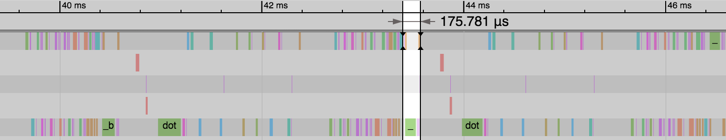
We can see a huge reduction in the time taken for the backward pass and parameter update step: 3.99ms vs 0.18ms. And this reduces the overall time of the epoch significantly. Our gradient consumes a much smaller amount of memory and means only a subset of parameters need updating as part of the sgd_update step. Some optimizers don’t support sparse gradients however, so reference the specific optimizer’s documentation for more details.
print_memory_allocation(net, block_idxs=[0, 2, 4])
Memory Allocation for Weight:
512.000 MBs ( 99.999%) for fullyconnectedsparse1
  0.004 MBs (  0.001%) for fullyconnected2
  0.000 MBs (  0.000%) for fullyconnected3
Memory Allocation for Weight Gradient:
  0.059 MBs ( 93.490%) for fullyconnectedsparse1
  0.004 MBs (  6.460%) for fullyconnected2
  0.000 MBs (  0.050%) for fullyconnected3
Advanced: Sparse weight
You can optimize this example further by setting the weight’s stype to 'row_sparse', but whether 'row_sparse' weights make sense or not will depends on your specific task. See contrib.SparseEmbedding for an example of this.
Conclusion
As part of this tutorial, we learned how to write sparse data to disk in LibSVM format and load it back in sparse batches with the LibSVMIter. We learned how to improve the performance of Gluon’s nn.Dense on sparse arrays using mx.nd.sparse. And lastly, we set grad_stype to 'row_sparse' to reduce the size of the gradient and speed up the parameter
update step.
Recommended Next Steps
More detail on the CSRNDArray sparse array format can be found in this tutorial.
More detail on the RowSparseNDArray sparse array format can be found in this tutorial.
Users of the Module API can see a symbolic only example in this tutorial.