Quantize with MKL-DNN backend
This document is to introduce how to quantize the customer models from FP32 to INT8 with Apache/MXNet toolkit and APIs under Intel CPU.
If you are not familiar with Apache/MXNet quantization flow, please reference quantization blog first, and the performance data is shown in Apache/MXNet C++ interface and GluonCV.
Installation and Prerequisites
Installing MXNet with MKLDNN backend is an easy and essential process. You can follow How to build and install MXNet with MKL-DNN backend to build and install MXNet from source. Also, you can install the release or nightly version via PyPi and pip directly by running:
# release version
pip install mxnet

# latest nightly development version
pip install --pre "mxnet<2" -f https://dist.mxnet.io/python
Image Classification Demo
A quantization script imagenet_gen_qsym_mkldnn.py has been designed to launch quantization for image-classification models. This script is integrated with Gluon-CV modelzoo, so that all pre-trained models can be downloaded from Gluon-CV and then converted for quantization. For details, you can refer Model Quantization with Calibration Examples.
Integrate Quantization Flow to Your Project
Quantization flow works for both symbolic and Gluon models. If you’re using Gluon, you can first refer Saving and Loading Gluon Models to hybridize your computation graph and export it as a symbol before running quantization.
In general, the quantization flow includes 4 steps. The user can get the acceptable accuracy from step 1 to 3 with minimum effort. Most of thing in this stage is out-of-box and the data scientists and researchers only need to focus on how to represent data and layers in their model. After a quantized model is generated, you may want to deploy it online and the performance will be the next key point. Thus, step 4, calibration, can improve the performance a lot by reducing lots of runtime calculation.

Now, we are going to take Gluon ResNet18 as an example to show how each step work.
Initialize Model
import logging
import mxnet as mx
from mxnet.gluon.model_zoo import vision
from mxnet.contrib.quantization import *

logging.basicConfig()
logger = logging.getLogger('logger')
logger.setLevel(logging.INFO)

batch_shape = (1, 3, 224, 224)
resnet18 = vision.resnet18_v1(pretrained=True)
resnet18.hybridize()
resnet18.forward(mx.nd.zeros(batch_shape))
resnet18.export('resnet18_v1')
sym, arg_params, aux_params = mx.model.load_checkpoint('resnet18_v1', 0)
# (optional) visualize float32 model
mx.viz.plot_network(sym)
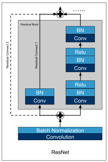
First, we download resnet18-v1 model from gluon modelzoo and export it as a symbol. You can visualize float32 model. Below is a raw residual block.
Model Fusion
sym = sym.get_backend_symbol('MKLDNN_QUANTIZE')
# (optional) visualize fused float32 model
mx.viz.plot_network(sym)
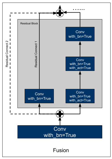
It’s important to add this line to enable graph fusion before quantization to get better performance. Below is a fused residual block. Batchnorm, Activation and elemwise_add are fused into Convolution.
Quantize Model
A python interface quantize_graph is provided for the user. Thus, it is very flexible for the data scientist to construct the expected models based on different requirements in a real deployment.
# quantize configs
# set exclude layers
excluded_names = []
# set calib mode.
calib_mode = 'none'
# set calib_layer
calib_layer = None
# set quantized_dtype
quantized_dtype = 'auto'
logger.info('Quantizing FP32 model Resnet18-V1')
qsym, qarg_params, aux_params, collector = quantize_graph(sym=sym, arg_params=arg_params, aux_params=aux_params,
                                                          excluded_sym_names=excluded_names,
                                                          calib_mode=calib_mode, calib_layer=calib_layer,
                                                          quantized_dtype=quantized_dtype, logger=logger)
# (optional) visualize quantized model
mx.viz.plot_network(qsym)
# save quantized model
mx.model.save_checkpoint('quantized-resnet18_v1', 0, qsym, qarg_params, aux_params)
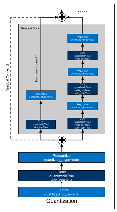
By applying quantize_graph to the symbolic model, a new quantized model can be generated, named qsym along with its parameters. We can see _contrib_requantize operators are inserted after Convolution to convert the INT32 output to FP32.
Below table gives some descriptions.
param |
type |
description |
|---|---|---|
excluded _sym_names |
list of strings |
A list of strings representing the names of the symbols that users want to excluding from being quantized. |
calib_mode |
str |
If calib_mode=‘none’, no calibration will be used and the thresholds for requantization after the corresponding layers will be calculated at runtime by calling min and max operators. The quantized models generated in this mode are normally 10-20% slower than those with calibrations during inference.If calib_mode=‘naive’, the min and max values of the layer outputs from a calibration dataset will be directly taken as the thresholds for quantization.If calib_mode=‘entropy’, the thresholds for quantization will be derived such that the KL divergence between the distributions of FP32 layer outputs and quantized layer outputs is minimized based upon the calibration dataset. |
c alib_layer |
function |
Given a layer’s output name in string, return True or False for deciding whether to calibrate this layer.If yes, the statistics of the layer’s output will be collected; otherwise, no information of the layer’s output will be collected.If not provided, all the layers’ outputs that need requantization will be collected. |
quant ized_dtype |
str |
The quantized destination type for input data. Currently support ‘int8’, ‘uint8’ and ‘auto’.‘auto’ means automatically select output type according to calibration result. |
Evaluate & Tune
Now, you get a pair of quantized symbol and params file for inference. For Gluon inference, only difference is to load model and params by a SymbolBlock as below example:
quantized_net = mx.gluon.SymbolBlock.imports('quantized-resnet18_v1-symbol.json', 'data', 'quantized-resnet18_v1-0000.params')
quantized_net.hybridize(static_shape=True, static_alloc=True)
batch_size = 1
data = mx.nd.ones((batch_size,3,224,224))
quantized_net(data)
Now, you can get the accuracy from a quantized network. Furthermore, you can try to select different layers or OPs to be quantized by excluded_sym_names parameter and figure out an acceptable accuracy.
Calibrate Model (optional for performance)
The quantized model generated in previous steps can be very slow during inference since it will calculate min and max at runtime. We recommend using offline calibration for better performance by setting calib_mode to naive or entropy. And then calling set_monitor_callback api to collect layer information with a subset of the validation datasets before int8 inference.
# quantization configs
# set exclude layers
excluded_names = []
# set calib mode.
calib_mode = 'naive'
# set calib_layer
calib_layer = None
# set quantized_dtype
quantized_dtype = 'auto'
logger.info('Quantizing FP32 model resnet18-V1')
cqsym, cqarg_params, aux_params, collector = quantize_graph(sym=sym, arg_params=arg_params, aux_params=aux_params,
                                                          excluded_sym_names=excluded_names,
                                                          calib_mode=calib_mode, calib_layer=calib_layer,
                                                          quantized_dtype=quantized_dtype, logger=logger)

# download imagenet validation dataset
mx.test_utils.download('http://data.mxnet.io/data/val_256_q90.rec', 'dataset.rec')
# set rgb info for data
mean_std = {'mean_r': 123.68, 'mean_g': 116.779, 'mean_b': 103.939, 'std_r': 58.393, 'std_g': 57.12, 'std_b': 57.375}
# set batch size
batch_size = 16
# create DataIter
data = mx.io.ImageRecordIter(path_imgrec='dataset.rec', batch_size=batch_size, data_shape=batch_shape[1:], rand_crop=False, rand_mirror=False, **mean_std)
# create module
mod = mx.mod.Module(symbol=sym, label_names=None, context=mx.cpu())
mod.bind(for_training=False, data_shapes=data.provide_data, label_shapes=None)
mod.set_params(arg_params, aux_params)

# calibration configs
# set num_calib_batches
num_calib_batches = 5
max_num_examples = num_calib_batches * batch_size
# monitor FP32 Inference
mod._exec_group.execs[0].set_monitor_callback(collector.collect, monitor_all=True)
num_batches = 0
num_examples = 0
for batch in data:
    mod.forward(data_batch=batch, is_train=False)
    num_batches += 1
    num_examples += batch_size
    if num_examples >= max_num_examples:
        break
if logger is not None:
    logger.info("Collected statistics from %d batches with batch_size=%d"
                % (num_batches, batch_size))
After that, layer information will be filled into the collector returned by quantize_graph api. Then, you need to write the layer information into int8 model by calling calib_graph api.
# write scaling factor into quantized symbol
cqsym, cqarg_params, aux_params = calib_graph(qsym=cqsym, arg_params=arg_params, aux_params=aux_params,
                                            collector=collector, calib_mode=calib_mode,
                                            quantized_dtype=quantized_dtype, logger=logger)
# (optional) visualize quantized model
mx.viz.plot_network(cqsym)
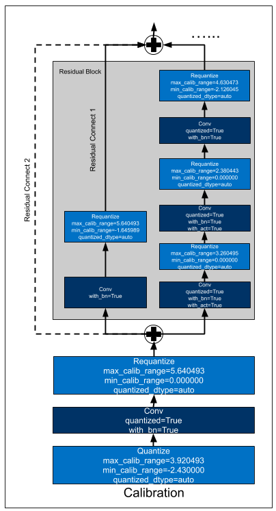
Below is a quantized residual block with naive calibration. We can see min_calib_range and max_calib_range are written into _contrib_requantize operators.
When you get a quantized model with calibration, keeping sure to call fusion api again since this can fuse some requantize or dequantize operators for further performance improvement.
# perform post-quantization fusion
cqsym = cqsym.get_backend_symbol('MKLDNN_QUANTIZE')
# (optional) visualize post-quantized model
mx.viz.plot_network(cqsym)
# save quantized model
mx.model.save_checkpoint('quantized-resnet18_v1', 0, cqsym, cqarg_params, aux_params)
Below is a post-quantized residual block. We can see _contrib_requantize operators are fused into Convolution operators.

BTW, You can also modify the min_calib_range and max_calib_range in the JSON file directly.
    {
      "op": "_sg_mkldnn_conv",
      "name": "quantized_sg_mkldnn_conv_bn_act_6",
      "attrs": {
        "max_calib_range": "3.562147",
        "min_calib_range": "0.000000",
        "quantized": "true",
        "with_act": "true",
        "with_bn": "true"
      },
......
Tips for Model Calibration
Accuracy Tuning
Try to use
entropycalib mode;Try to exclude some layers which may cause obvious accuracy drop;
Change calibration dataset by setting different
num_calib_batchesor shuffle your validation dataset;Use Intel® Neural Compressor (see below)
Performance Tuning
Keep sure to perform graph fusion before quantization;
If lots of
requantizelayers exist, keep sure to perform post-quantization fusion after calibration;Compare the MXNet profile or
MKLDNN_VERBOSEof float32 and int8 inference;
Deploy with Python/C++
MXNet also supports deploy quantized models with C++. Refer MXNet C++ Package for more details.
Improving accuracy with Intel® Neural Compressor
The accuracy of a model can decrease as a result of quantization. When the accuracy drop is significant, we can try to manually find a better quantization configuration (exclude some layers, try different calibration methods, etc.), but for bigger models this might prove to be a difficult and time consuming task. Intel® Neural Compressor (INC) tries to automate this process using several tuning heuristics, which aim to find the quantization configuration that satisfies the specified accuracy requirement.
NOTE:
Most tuning strategies will try different configurations on an evaluation dataset in order to find out how each layer affects the accuracy of the model. This means that for larger models, it may take a long time to find a solution (as the tuning space is usually larger and the evaluation itself takes longer).
Installation and Prerequisites
Install MXNet with MKLDNN enabled as described in the previous section.
Install Intel® Neural Compressor:
Use one of the commands below to install INC (supported python versions are: 3.6, 3.7, 3.8, 3.9):
# install stable version from pip
pip install neural-compressor

# install nightly version from pip
pip install -i https://test.pypi.org/simple/ neural-compressor

# install stable version from conda
conda install neural-compressor -c conda-forge -c intel
Configuration file
Quantization tuning process can be customized in the yaml configuration file. Below is a simple example:
# cnn.yaml

version: 1.0

model:
  name: cnn
  framework: mxnet

quantization:
  calibration:
    sampling_size: 160 # number of samples for calibration

tuning:
  strategy:
    name: basic
  accuracy_criterion:
    relative: 0.01
  exit_policy:
    timeout: 0
  random_seed: 9527
We are using the basic strategy, but you could also try out different ones. Here you can find a list of strategies available in INC and details of how they work. You can also add your own strategy if the existing ones do not suit your needs.
Since the value of timeout is 0, INC will run until it finds a configuration that satisfies the accuracy criterion and then exit. Depending on the strategy this may not be ideal, as sometimes it would be better to further explore the tuning space to find a superior configuration both in terms of accuracy and speed. To achieve this, we can set a specific timeout value, which will tell INC how long (in seconds) it should run.
For more information about the configuration file, see the template from the official INC repo. Keep in mind that only the post training quantization is currently supported for MXNet.
Model quantization and tuning
In general, Intel® Neural Compressor requires 4 elements in order to run: 1. Config file - like the example above 2. Model to be quantized 3. Calibration dataloader 4. Evaluation function - a function that takes a model as an argument and returns the accuracy it achieves on a certain evaluation dataset.
Quantizing ResNet
The previous sections described how to quantize ResNet using the native MXNet quantization. This example shows how we can achieve the same (with the auto-tuning) using INC.
Get the model
import logging
import mxnet as mx
from mxnet.gluon.model_zoo import vision

logging.basicConfig()
logger = logging.getLogger('logger')
logger.setLevel(logging.INFO)

batch_shape = (1, 3, 224, 224)
resnet18 = vision.resnet18_v1(pretrained=True)
Prepare the dataset:
mx.test_utils.download('http://data.mxnet.io/data/val_256_q90.rec', 'data/val_256_q90.rec')

batch_size = 16
mean_std = {'mean_r': 123.68, 'mean_g': 116.779, 'mean_b': 103.939,
            'std_r': 58.393, 'std_g': 57.12, 'std_b': 57.375}

data = mx.io.ImageRecordIter(path_imgrec='data/val_256_q90.rec',
                             batch_size=batch_size,
                             data_shape=batch_shape[1:],
                             rand_crop=False,
                             rand_mirror=False,
                             shuffle=False,
                             **mean_std)
data.batch_size = batch_size
Prepare the evaluation function:
eval_samples = batch_size*10

def eval_func(model):
    data.reset()
    metric = mx.metric.Accuracy()
    for i, batch in enumerate(data):
        if i * batch_size >= eval_samples:
            break
        x = batch.data[0].as_in_context(mx.cpu())
        label = batch.label[0].as_in_context(mx.cpu())
        outputs = model.forward(x)
        metric.update(label, outputs)
    return metric.get()[1]
Run Intel® Neural Compressor:
from neural_compressor.experimental import Quantization
quantizer = Quantization("./cnn.yaml")
quantizer.model = resnet18
quantizer.calib_dataloader = data
quantizer.eval_func = eval_func
qnet = quantizer.fit().model
Since this model already achieves good accuracy using native quantization (less than 1% accuracy drop), for the given configuration file, INC will end on the first configuration, quantizing all layers using naive calibration mode for each. To see the true potential of INC, we need a model which suffers from a larger accuracy drop after quantization.
Quantizing BERT
This example shows how to use INC to quantize BERT-base for MRPC. In this case, the native MXNet quantization usually introduce a significant accuracy drop (2% - 5% using naive calibration mode). To simplify the code, model and task specific boilerplate has been moved to the details.py file.
This is the configuration file for this example:
version: 1.0

model:
  name: bert
  framework: mxnet

quantization:
  calibration:
    sampling_size: 320 # number of samples for calibration

tuning:
  strategy:
    name: basic
  accuracy_criterion:
    relative: 0.01
  exit_policy:
    timeout: 0
    max_trials: 9999 # default is 100
  random_seed: 9527
And here is the script:
from pathlib import Path
from functools import partial

import details
from neural_compressor.experimental import Quantization, common

# constants
INC_CONFIG_PATH = Path('./bert.yaml').resolve()
PARAMS_PATH = Path('./bert_mrpc.params').resolve()
OUTPUT_DIR_PATH = Path('./output/').resolve()
OUTPUT_MODEL_PATH = OUTPUT_DIR_PATH/'quantized_model'
OUTPUT_DIR_PATH.mkdir(parents=True, exist_ok=True)

# Prepare the dataloaders (calib_dataloader is same as train_dataloader but without shuffling)
train_dataloader, dev_dataloader, calib_dataloader = details.preprocess_data()

# Get the model
model = details.BERTModel(details.BACKBONE, dropout=0.1, num_classes=details.NUM_CLASSES)
model.hybridize(static_alloc=True)

# finetune or load the parameters of already finetuned model
if not PARAMS_PATH.exists():
    model = details.finetune(model, train_dataloader, dev_dataloader, OUTPUT_DIR_PATH)
    model.save_parameters(str(PARAMS_PATH))
else:
    model.load_parameters(str(PARAMS_PATH), ctx=details.CTX, cast_dtype=True)

# run INC
calib_dataloader.batch_size = details.BATCH_SIZE
eval_func = partial(details.evaluate, dataloader=dev_dataloader)

quantizer = Quantization(str(INC_CONFIG_PATH))  # 1. Config file
quantizer.model = common.Model(model)           # 2. Model to be quantized
quantizer.calib_dataloader = calib_dataloader   # 3. Calibration dataloader
quantizer.eval_func = eval_func                 # 4. Evaluation function
quantized_model = quantizer.fit().model

# save the quantized model
quantized_model.export(str(OUTPUT_MODEL_PATH))
With the evaluation function hidden in the details.py file:
def evaluate(model, dataloader):
    metric = METRIC()
    for batch in dataloader:
        input_ids, segment_ids, valid_length, label = batch
        input_ids = input_ids.as_in_context(CTX)
        segment_ids = segment_ids.as_in_context(CTX)
        valid_length = valid_length.as_in_context(CTX)
        label = label.as_in_context(CTX).reshape((-1))

        out = model(input_ids, segment_ids, valid_length)
        metric.update([label], [out])

    metric_name, metric_val = metric.get()
    return metric_val
For comparision, this is how one could quantize this model using MXNet native quantization (this function is also located in the details.py file):
def native_quantization(model, calib_dataloader, dev_dataloader):
    quantized_model = quantize_net_v2(model,
                                      quantize_mode='smart',
                                      calib_data=calib_dataloader,
                                      calib_mode='naive',
                                      num_calib_examples=BATCH_SIZE*10)
    print('Native quantization results: {}'.format(evaluate(quantized_model, dev_dataloader)))
    return quantized_model
For complete code, see this example on the official GitHub repository.
Results:
Environment: - c6i.16xlarge Amazon EC2 instance (Intel(R) Xeon(R) Platinum 8375C CPU @ 2.90GHz) - Ubuntu 20.04 LTS - MXNet 1.9 - INC 1.9.1
Results on the validation dataset:
Quantization method |
Accuracy |
F1 |
Relative accuracy loss [%] |
Calibration/tuning time [s] |
Speedup |
|---|---|---|---|---|---|
No quantization (f32) |
0.8529 |
0.8956 |
0 |
0 |
1.0 |
Native ‘naive’, 10 batches |
0.8259 |
0.8775 |
3.1657 |
31 |
1.3811 |
Native ‘naive’, 20 batches |
0.8210 |
0.8731 |
3.7402 |
58 |
1.3866 |
Native ‘entropy’, 10 batches |
0.8064 |
0.8557 |
5.4520 |
37 |
1.3789 |
Native ‘entropy’, 20 batches |
0.8137 |
0.8624 |
4.5961 |
67 |
1.3460 |
INC, ‘basic’ |
0.8456 |
0.8889 |
0.8559 |
197 |
1.4418 |
INC, ‘bayesian’ |
0.8529 |
0.8888 |
0 |
129 |
1.4275 |
INC, ‘mse’ |
0.8480 |
0.8954 |
0.5745 |
974 |
0.9642 |
All INC strategies found configurations meeting the 1% relative accuracy loss criterion. Only the mse strategy struggled, taking the longest time and generating configuration that is slower than the f32 model. Although these results may suggest that the mse strategy is the worst and the bayesian strategy is the best, different strategies may give better results for specific models and tasks. Usually the basic strategy is the most stable one.
Here is an example of a configuration generated by INC with the basic strategy:
Layers quantized using min-max (
naive) calibration algorithm:{'bertclassifier0_dropout0_fwd', 'bertencoder0_layernorm0_layernorm0', 'bertencoder0_transformer0_dotproductselfattentioncell0_dropout0_fwd', 'bertencoder0_transformer0_dotproductselfattentioncell0_reshape3', 'bertencoder0_transformer0_dotproductselfattentioncell0_reshape7', 'bertencoder0_transformer0_layernorm0_layernorm0', 'bertencoder0_transformer0_positionwiseffn0_layernorm0_layernorm0', 'bertencoder0_transformer10_dotproductselfattentioncell0_dropout0_fwd', 'bertencoder0_transformer10_dotproductselfattentioncell0_reshape3', 'bertencoder0_transformer10_dotproductselfattentioncell0_reshape7', 'bertencoder0_transformer10_layernorm0_layernorm0', 'bertencoder0_transformer10_positionwiseffn0_layernorm0_layernorm0', 'bertencoder0_transformer11_dotproductselfattentioncell0_dropout0_fwd', 'bertencoder0_transformer11_dotproductselfattentioncell0_reshape3', 'bertencoder0_transformer11_dotproductselfattentioncell0_reshape7', 'bertencoder0_transformer11_layernorm0_layernorm0', 'bertencoder0_transformer1_dotproductselfattentioncell0_dropout0_fwd', 'bertencoder0_transformer1_dotproductselfattentioncell0_reshape3', 'bertencoder0_transformer1_dotproductselfattentioncell0_reshape7', 'bertencoder0_transformer1_layernorm0_layernorm0', 'bertencoder0_transformer1_positionwiseffn0_layernorm0_layernorm0', 'bertencoder0_transformer2_dotproductselfattentioncell0_dropout0_fwd', 'bertencoder0_transformer2_dotproductselfattentioncell0_reshape3', 'bertencoder0_transformer2_dotproductselfattentioncell0_reshape7', 'bertencoder0_transformer2_layernorm0_layernorm0', 'bertencoder0_transformer2_positionwiseffn0_layernorm0_layernorm0', 'bertencoder0_transformer3_dotproductselfattentioncell0_dropout0_fwd', 'bertencoder0_transformer3_dotproductselfattentioncell0_reshape3', 'bertencoder0_transformer3_dotproductselfattentioncell0_reshape7', 'bertencoder0_transformer3_layernorm0_layernorm0', 'bertencoder0_transformer3_positionwiseffn0_layernorm0_layernorm0', 'bertencoder0_transformer4_dotproductselfattentioncell0_dropout0_fwd', 'bertencoder0_transformer4_dotproductselfattentioncell0_reshape3', 'bertencoder0_transformer4_dotproductselfattentioncell0_reshape7', 'bertencoder0_transformer4_layernorm0_layernorm0', 'bertencoder0_transformer4_positionwiseffn0_layernorm0_layernorm0', 'bertencoder0_transformer5_dotproductselfattentioncell0_dropout0_fwd', 'bertencoder0_transformer5_dotproductselfattentioncell0_reshape3', 'bertencoder0_transformer5_dotproductselfattentioncell0_reshape7', 'bertencoder0_transformer5_layernorm0_layernorm0', 'bertencoder0_transformer5_positionwiseffn0_layernorm0_layernorm0', 'bertencoder0_transformer6_dotproductselfattentioncell0_dropout0_fwd', 'bertencoder0_transformer6_dotproductselfattentioncell0_reshape3', 'bertencoder0_transformer6_dotproductselfattentioncell0_reshape7', 'bertencoder0_transformer6_layernorm0_layernorm0', 'bertencoder0_transformer6_positionwiseffn0_layernorm0_layernorm0', 'bertencoder0_transformer7_dotproductselfattentioncell0_dropout0_fwd', 'bertencoder0_transformer7_dotproductselfattentioncell0_reshape3', 'bertencoder0_transformer7_dotproductselfattentioncell0_reshape7', 'bertencoder0_transformer7_layernorm0_layernorm0', 'bertencoder0_transformer7_positionwiseffn0_layernorm0_layernorm0', 'bertencoder0_transformer8_dotproductselfattentioncell0_dropout0_fwd', 'bertencoder0_transformer8_dotproductselfattentioncell0_reshape3', 'bertencoder0_transformer8_dotproductselfattentioncell0_reshape7', 'bertencoder0_transformer8_layernorm0_layernorm0', 'bertencoder0_transformer8_positionwiseffn0_layernorm0_layernorm0', 'bertencoder0_transformer9_dotproductselfattentioncell0_dropout0_fwd', 'bertencoder0_transformer9_dotproductselfattentioncell0_reshape3', 'bertencoder0_transformer9_dotproductselfattentioncell0_reshape7', 'bertencoder0_transformer9_layernorm0_layernorm0', 'bertencoder0_transformer9_positionwiseffn0_layernorm0_layernorm0', 'bertmodel0_reshape0', 'sg_mkldnn_fully_connected_0', 'sg_mkldnn_fully_connected_1', 'sg_mkldnn_fully_connected_11', 'sg_mkldnn_fully_connected_12', 'sg_mkldnn_fully_connected_13', 'sg_mkldnn_fully_connected_15', 'sg_mkldnn_fully_connected_16', 'sg_mkldnn_fully_connected_17', 'sg_mkldnn_fully_connected_19', 'sg_mkldnn_fully_connected_20', 'sg_mkldnn_fully_connected_21', 'sg_mkldnn_fully_connected_23', 'sg_mkldnn_fully_connected_24', 'sg_mkldnn_fully_connected_25', 'sg_mkldnn_fully_connected_27', 'sg_mkldnn_fully_connected_28', 'sg_mkldnn_fully_connected_29', 'sg_mkldnn_fully_connected_3', 'sg_mkldnn_fully_connected_31', 'sg_mkldnn_fully_connected_32', 'sg_mkldnn_fully_connected_33', 'sg_mkldnn_fully_connected_35', 'sg_mkldnn_fully_connected_36', 'sg_mkldnn_fully_connected_37', 'sg_mkldnn_fully_connected_39', 'sg_mkldnn_fully_connected_4', 'sg_mkldnn_fully_connected_40', 'sg_mkldnn_fully_connected_41', 'sg_mkldnn_fully_connected_43', 'sg_mkldnn_fully_connected_44', 'sg_mkldnn_fully_connected_45', 'sg_mkldnn_fully_connected_47', 'sg_mkldnn_fully_connected_48', 'sg_mkldnn_fully_connected_49', 'sg_mkldnn_fully_connected_5', 'sg_mkldnn_fully_connected_7', 'sg_mkldnn_fully_connected_8', 'sg_mkldnn_fully_connected_9', 'sg_mkldnn_fully_connected_eltwise_10', 'sg_mkldnn_fully_connected_eltwise_14', 'sg_mkldnn_fully_connected_eltwise_18', 'sg_mkldnn_fully_connected_eltwise_2', 'sg_mkldnn_fully_connected_eltwise_22', 'sg_mkldnn_fully_connected_eltwise_26', 'sg_mkldnn_fully_connected_eltwise_30', 'sg_mkldnn_fully_connected_eltwise_34', 'sg_mkldnn_fully_connected_eltwise_38', 'sg_mkldnn_fully_connected_eltwise_42', 'sg_mkldnn_fully_connected_eltwise_46', 'sg_mkldnn_fully_connected_eltwise_6'}Layers quantized using KL (
entropy) calibration algorithm:{'sg_mkldnn_selfatt_qk_0', 'sg_mkldnn_selfatt_qk_10', 'sg_mkldnn_selfatt_qk_12', 'sg_mkldnn_selfatt_qk_14', 'sg_mkldnn_selfatt_qk_16', 'sg_mkldnn_selfatt_qk_18', 'sg_mkldnn_selfatt_qk_2', 'sg_mkldnn_selfatt_qk_20', 'sg_mkldnn_selfatt_qk_22', 'sg_mkldnn_selfatt_qk_4', 'sg_mkldnn_selfatt_qk_6', 'sg_mkldnn_selfatt_qk_8', 'sg_mkldnn_selfatt_valatt_1', 'sg_mkldnn_selfatt_valatt_11', 'sg_mkldnn_selfatt_valatt_13', 'sg_mkldnn_selfatt_valatt_15', 'sg_mkldnn_selfatt_valatt_17', 'sg_mkldnn_selfatt_valatt_19', 'sg_mkldnn_selfatt_valatt_21', 'sg_mkldnn_selfatt_valatt_23', 'sg_mkldnn_selfatt_valatt_3', 'sg_mkldnn_selfatt_valatt_5', 'sg_mkldnn_selfatt_valatt_7', 'sg_mkldnn_selfatt_valatt_9'}Layers excluded from quantization:
{'sg_mkldnn_fully_connected_43'}
Tips
In order to get a solution that generalizes well, evaluate the model (in eval_func) on a representative dataset.
With
history.snapshotfile (generated by INC) you can recover any model that was generated during the tuning process:from neural_compressor.utils.utility import recover quantized_model = recover(f32_model, 'nc_workspace/<tuning date>/history.snapshot', configuration_idx).model