Why MXNet came to be?
Why was MXNet developed in the first place ?
Probably, if you've stumbled upon this page, you've heard of deep learning. Deep learning denotes the modern incarnation of neural networks, and it's the technology behind recent breakthroughs in self-driving cars, machine translation, speech recognition and more. While widespread interest in deep learning took off in 2012, deep learning has become an indispensable tool for countless industries.
It might not come as a surprise that researchers have investigated neural networks for decades. Warren McCulloch and Walter Pitts suggested the forerunner of today's artificial neurons back in 1943. Each neuron is connected to other neurons along edges, analogous to the synapses that connect real neurons. And associated with each edge is a weight that indicates whether the connection is excitatory or inhibitatory and the strength of the connection.
In the 1980s, the modern version of neural networks took shape. Researchers arranged artificial neurons into layers. Neurons in any layer get input from the neurons in the layers below them. And, in turn, their output feeds into the neurons in the layer above. Typically, the lowest layer represents the input to a neural network. After computing the values of each layer, the output values are read out from the topmost layer. The behavior of the network is determined by the setting of the weights. And the process of learning in neural networks is precisely the process of searching for good settings of these weights.
All that we need is an algorithm that tells us how to perform this search. And since David Rumelhart and colleagues introduced the backpropagation learning algorithm to train neural networks, nearly all the major ideas have been in place. Still, for many years neural networks took a backseat to classical statistical methods like logistic regression and support vector machines (SVMs). So you might reasonably ask, what's changed to garner such interest?
Scale and Computation
The two biggest factors driving innovation in deep learning now are data and computation. With distributed cloud computing and parallelism across GPU cores, we can train models millions of times faster than researchers could in the 1980s. The availability of large, high-quality datasets is another factor driving the field forward. In the 1990s, the best datasets in computer vision had thousands of low-resolution images and ground truth assignments to a small number of classes. Today, researchers cut their teeth on ImageNet, a massive dataset containing millions of high-resolution images from a thousand distinct classes. The falling price of storage and high network bandwidth make it affordable to work with big data at will.
In this new world, with bigger datasets and abundant computation, neural networks dominate on most pattern recognition problems. Over the last five years, neural networks have come to dominate on nearly every problem in computer vision, replacing classical models and hand-engineered features. Similarly, nearly every production speech recognition system now relies on neural networks, where replacing the hidden Markov models that previously held sway.
While GPUs and clusters present a huge opportunity for accelerating neural network training, adapting traditional machine learning code to take advantage of these resources can be challenging. The familiar scientific computing stacks (Matlab, R, or NumPy & SciPy) give no straight-forward way to exploit these distributed resources.
Acceleration libraries like MXNet offer powerful tools to help developers exploit the full capabilities of GPUs and cloud computing. While these tools are generally useful and applicable to any mathematical computation, MXNet places a special emphasis on speeding up the development and deployment of large-scale deep neural networks. In particular, we offer the following capabilities: * Device Placement: With MXNet, it's easy to specify where each data structures should live. * Multi-GPU training: MXNet makes it easy to scale computation with number of available GPUs. * Automatic differentiation: MXNet automates the derivative calculations that once bogged down neural network research. * Optimized Predefined Layers: While you can code up your own layers in MXNet, the predefined layers are optimized for speed, outperforming competing libraries.
Deep Nets on Fast Computers
While MXNet can accelerate any numerical computation, we developed the library with neural networks in mind. However you plan to use MXNet, neural networks make for a powerful motivating example to display MXNet's capabilities.
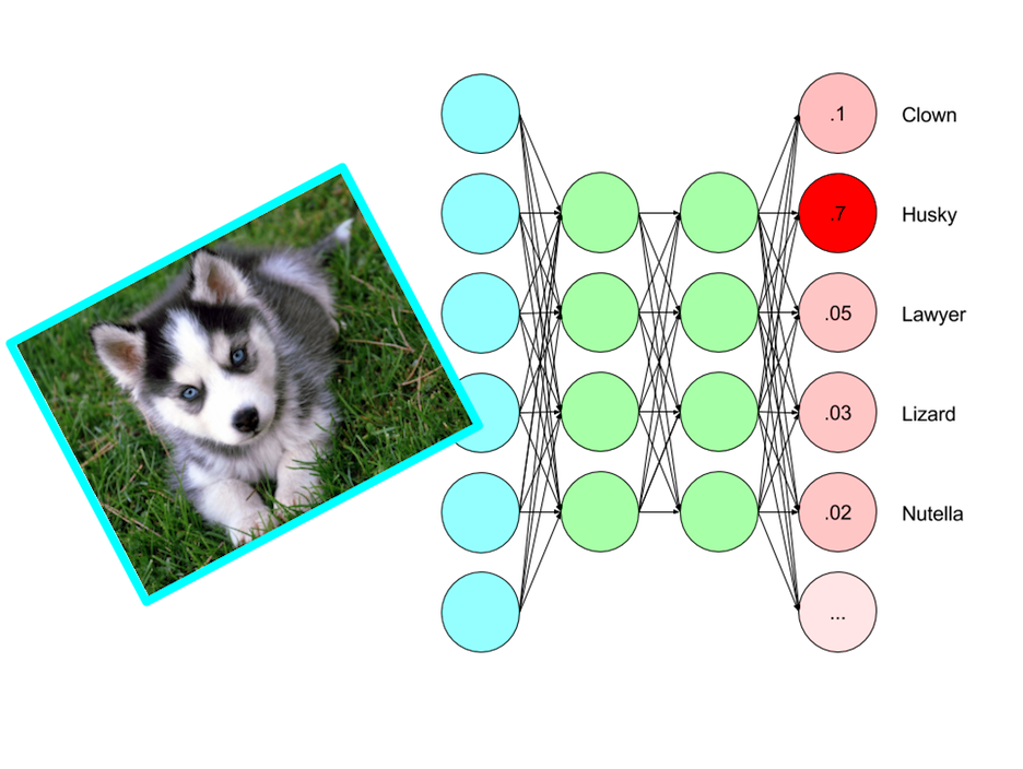
Neural networks are just functions for transforming input arrays X into output arrays Y.
In the case of image classification, X might represent the pixel values of an image, and Y might represent the corresponding probabilities that the image belongs to each of 10 classes.
For language translation, X and Y both might denote sequences of words. We'll revisit the way you might represent sequences in subsequent tutorials - so for now it's safe to think of X and Y as fixed length vectors.
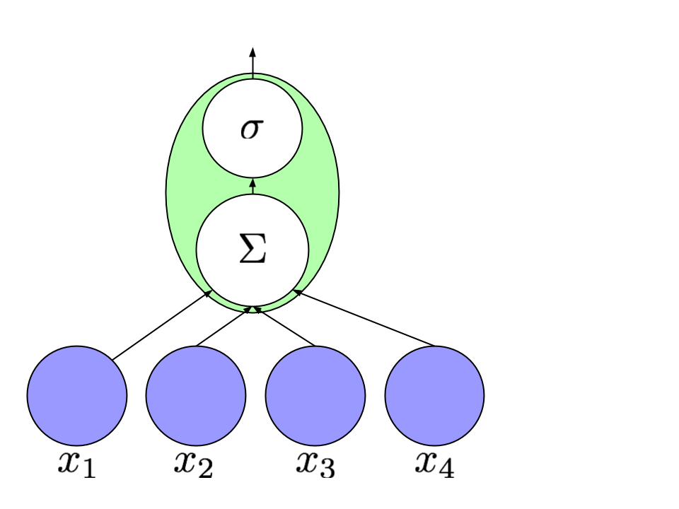
To perform this mapping, neural networks stack layers of computation. Each layer consists of a linear function followed by a nonlinear transformation. In MXNet we might express this as:
python
hidden_linear = mx.sym.dot(X, W)
hidden_activation = mx.sym.tanh(hidden_linear)
The linear transformations consist of multiplication by parameter arrays (W above).
When we talk about learning we mean finding the right set of values for W.
With just one layer, we can implement the familiar family of linear models,
including linear and logistic regression, linear support vector machines (SVMs), and the perceptron algorithm.
With more layers and a few clever constraints, we can implement all of today's state-of-the-art deep learning techniques.
Of course, tens or hundreds of matrix multiplications can be computationally taxing. Generally, these linear operations are the computational bottleneck. Fortunately, linear operators can be parallelized trivially across the thousands of cores on a GPU. But low-level GPU programming requires specialized skills that are not common even among leading researchers in the ML community. Moreover, even for CUDA experts, implementing a new neural network architecture shouldn't require weeks of programming to implement low-level linear algebra operations. That's where MXNet comes in. * MXNet provides optimized numerical computation for GPUs and distributed ecosystems, from the comfort of high-level environments like Python and R * MXNet automates common workflows, so standard neural networks can be expressed concisely in just a few lines of code
Now let's take a closer look at the computational demands of neural networks and give a sense of how MXNet helps us to write better, faster, code. Say we have a neural network trained to recognize spam from the content of emails. The emails may be streaming from an online service (at inference time), or from a large offline dataset D (at training time). In either case, the dataset typically must be managed by the CPU.
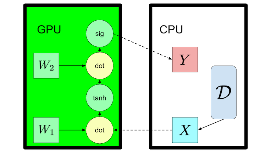
To compute the transformation of a neural network quickly, we need both the parameters and data points to make it into GPU memory. For any example X, the parameters W are the same. Moreover the size of the model tends to dwarf the size of an individual example. So we might arrive at the natural insight that parameters should always live on the GPU, even if the dataset itself must live on the CPU or stream in. This prevents IO from becoming the bottleneck during training or inference.
Fortunately, MXNet makes this kind of assignment easy.
import mxnet.ndarray as nd

X  = nd.zeros((10000, 40000), mx.cpu(0))           #Allocate an array to store 1000 datapoints (of 40k dimensions) that lives on the CPU
W1 = nd.zeros(shape=(40000, 1024), mx.gpu(0))      #Allocate a 40k x 1024 weight matrix on GPU for the 1st layer of the net
W2 = nd.zeros(shape=(1024, 10), mx.gpu(0))         #Allocate a 1024 x 1024 weight matrix on GPU for the 2nd layer of the net
Similarly, MXNet makes it easy to specify the computing device
with mx.Context(mx.gpu()):          # Absent this statement, by default, MXNet will execute on CPU
    h = nd.tanh(nd.dot(X, W1))
    y = nd.sigmoid(nd.dot(h1, W2))
Thus, with only a high-level understanding of how our numerical computation maps onto an execution environment, MXNet allows us to exert fine-grained control when needed.
Nuts and Bolts
MXNet supports two styles of programming: imperative programming (supported by the NDArray API) and symbolic programming (supported by the Symbol API). In short, imperative programming is the style that you're likely to be most familiar with. Here if A and B are variables denoting matrices, then C = A + B is a piece of code that when executed sums the values referenced by A and B and stores their sum C in a new variable. Symbolic programming, on the other hand, allows functions to be defined abstractly through computation graphs. In the symbolic style, we first express complex functions in terms of placeholder values. Then, we can execute these functions by binding them to real values.
Imperative Programming with NDArray
If you're familiar with NumPy, then the mechanics of NDArray should be old hat. Like the corresponding numpy.ndarray, mxnet.ndarray (mxnet.nd for short) allows us to represent and manipulate multi-dimensional, homogenous arrays of fixed-size components. Converting between the two is effortless:
# Create a numpy array from an mxnet NDArray
A_np = np.array([[0,1,2,3,4],[5,6,7,8,9]])
A_nd = nd.array(A)

# Convert back to a numpy array
A2_np = A_nd.asnumpy()
Other deep learning libraries tend to rely on NumPy exclusively for imperative programming and the syntax. So you might reasonably wonder, why do we need to bother with NDArray? Put simply, other libraries only reap the advantages of GPU computing when executing symbolic functions. By using NDArray, MXNet users can specify device context and run on GPUs. In other words, MXNet gives you access to the high-speed computation for imperative operations that Tensorflow and Theano only give for symbolic operations.
X = mx.nd.array([[1,2],[3,4]])
Y = mx.nd.array([[5,6],[7,8]])
result = X + Y
Symbolic Programming in MXNet
In addition to providing fast math operations through NDArray, MXNet provides an interface for defining operations abstractly via a computation graph.
With mxnet.symbol, we define operations abstractly in terms of place holders. For example, in the following code a and b stand in for real values that will be supplied at run time.
When we call c = a+b, no numerical computation is performed. This operation simply builds a graph that defines the relationship between a, b and c. In order to perform a real calculation, we need to bind c to real values.
a = mx.sym.Variable('a')
b = mx.sym.Variable('b')
c = a + b
executor = c.bind(mx.cpu(), {'a': X, 'b': Y})
result = executor.forward()
Symbolic computation is useful for several reasons. First, because we define a full computation graph before executing it, MXNet can perform sophisticated optimizations to eliminate unnecessary or repeated work. This tends to give better performance than imperative programming. Second, because we store the relationships between different variables in the computation graph, MXNet can then perform efficient auto-differentiation.
However Symbolic programming is error-prone and very slow to iterate with, as the graph needs to be computed before it is processed.
Gluon for briding the gap between the two
MXNet Gluon aims to bridge the gap between the imperative nature of MXNet and its symbolic capabilities and keep the advantages of both through hybridization.
Conclusions
Given its combination of high performance, clean code, access to a high-level API, and low-level control, MXNet stands out as a unique choice among deep learning frameworks.