Step 5: Datasets and DataLoader

One of the most critical steps for model training and inference is loading the data: without data you can’t do Machine Learning! In this tutorial you will use the Gluon API to define a Dataset and use a DataLoader to iterate through the dataset in mini-batches.

import mxnet as mx
import os
import time
import tarfile

Introduction to Datasets

Dataset objects are used to represent collections of data, and include methods to load and parse the data (that is often stored on disk). Gluon has a number of different Dataset classes for working with image data straight out-of-the-box, but you’ll use the ArrayDataset to introduce the idea of a Dataset.

You will first start by generating random data X (with 3 variables) and corresponding random labels y to simulate a typical supervised learning task. You will generate 10 samples and pass them all to the ArrayDataset.

mx.np.random.seed(42) # Fix the seed for reproducibility
X = mx.np.random.uniform(size=(10, 3))
y = mx.np.random.uniform(size=(10, 1))
dataset = mx.gluon.data.dataset.ArrayDataset(X, y)

A key feature of a Dataset is the ability to retrieve a single sample given an index. Our random data and labels were generated in memory, so this ArrayDataset doesn’t have to load anything from disk, but the interface is the same for all Dataset’s.

sample_idx = 4
sample = dataset[sample_idx]

assert len(sample) == 2
assert sample[0].shape == (3, )
assert sample[1].shape == (1, )
print(sample)

(array([0.74707687, 0.37641123, 0.46362457]), array([0.35440788]))

[03:52:14] /work/mxnet/src/storage/storage.cc:202: Using Pooled (Naive) StorageManager for CPU

You get a tuple of a data sample and its corresponding label, which makes sense because you passed the data X and the labels y in that order when you instantiated the ArrayDataset. You don’t usually retrieve individual samples from Dataset objects though (unless you’re quality checking the output samples). Instead you use a DataLoader.

Introduction to DataLoader

A DataLoader is used to create mini-batches of samples from a Dataset, and provides a convenient iterator interface for looping these batches. It’s typically much more efficient to pass a mini-batch of data through a neural network than a single sample at a time, because the computation can be performed in parallel. A required parameter of DataLoader is the size of the mini-batches you want to create, called batch_size.

Another benefit of using DataLoader is the ability to easily load data in parallel using multiprocessing. You can set the num_workers parameter to the number of CPUs available on your machine for maximum performance, or limit it to a lower number to spare resources.

from multiprocessing import cpu_count
CPU_COUNT = cpu_count()

data_loader = mx.gluon.data.DataLoader(dataset, batch_size=5, num_workers=CPU_COUNT)

for X_batch, y_batch in data_loader:
    print("X_batch has shape {}, and y_batch has shape {}".format(X_batch.shape, y_batch.shape))

X_batch has shape (5, 3), and y_batch has shape (5, 1)
X_batch has shape (5, 3), and y_batch has shape (5, 1)

You can see 2 mini-batches of data (and labels), each with 5 samples, which makes sense given that you started with a dataset of 10 samples. When comparing the shape of the batches to the samples returned by the Dataset,you’ve gained an extra dimension at the start which is sometimes called the batch axis.

Our data_loader loop will stop when every sample of dataset has been returned as part of a batch. Sometimes the dataset length isn’t divisible by the mini-batch size, leaving a final batch with a smaller number of samples. DataLoader’s default behavior is to return this smaller mini-batch, but this can be changed by setting the last_batch parameter to discard (which ignores the last batch) or rollover (which starts the next epoch with the remaining samples).

Machine learning with Datasets and DataLoaders

You will often use a few different Dataset objects in your Machine Learning project. It’s essential to separate your training dataset from testing dataset, and it’s also good practice to have validation dataset (a.k.a. development dataset) that can be used for optimising hyperparameters.

Using Gluon Dataset objects, you define the data to be included in each of these separate datasets. It’s simple to create your own custom Dataset classes for other types of data. You can even use included Dataset objects for common datasets if you want to experiment quickly; they download and parse the data for you! In this example you use the Fashion MNIST dataset from Zalando Research.

Many of the image Dataset’s accept a function (via the optional transform parameter) which is applied to each sample returned by the Dataset. It’s useful for performing data augmentation, but can also be used for more simple data type conversion and pixel value scaling as seen below.

def transform(data, label):
    data = data.astype('float32')/255
    return data, label

train_dataset = mx.gluon.data.vision.datasets.FashionMNIST(train=True).transform(transform)
valid_dataset = mx.gluon.data.vision.datasets.FashionMNIST(train=False).transform(transform)

Downloading /home/jenkins_slave/.mxnet/datasets/fashion-mnist/train-images-idx3-ubyte.gz from https://apache-mxnet.s3-accelerate.dualstack.amazonaws.com/gluon/dataset/fashion-mnist/train-images-idx3-ubyte.gz...
Downloading /home/jenkins_slave/.mxnet/datasets/fashion-mnist/train-labels-idx1-ubyte.gz from https://apache-mxnet.s3-accelerate.dualstack.amazonaws.com/gluon/dataset/fashion-mnist/train-labels-idx1-ubyte.gz...
Downloading /home/jenkins_slave/.mxnet/datasets/fashion-mnist/t10k-images-idx3-ubyte.gz from https://apache-mxnet.s3-accelerate.dualstack.amazonaws.com/gluon/dataset/fashion-mnist/t10k-images-idx3-ubyte.gz...
Downloading /home/jenkins_slave/.mxnet/datasets/fashion-mnist/t10k-labels-idx1-ubyte.gz from https://apache-mxnet.s3-accelerate.dualstack.amazonaws.com/gluon/dataset/fashion-mnist/t10k-labels-idx1-ubyte.gz...

from matplotlib.pylab import imshow

sample_idx = 234
sample = train_dataset[sample_idx]
data = sample[0]
label = sample[1]
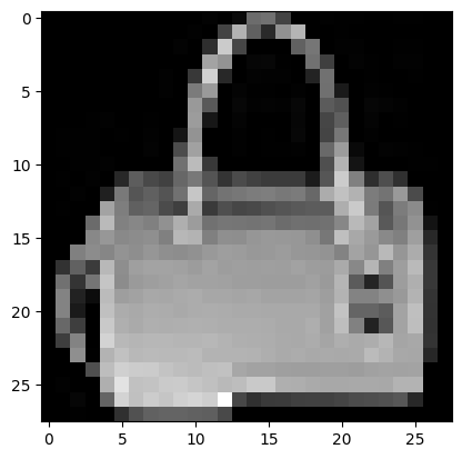
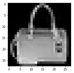
label_desc = {0:'T-shirt/top', 1:'Trouser', 2:'Pullover', 3:'Dress', 4:'Coat', 5:'Sandal', 6:'Shirt', 7:'Sneaker', 8:'Bag', 9:'Ankle boot'}

print("Data type: {}".format(data.dtype))
print("Label: {}".format(label))
print("Label description: {}".format(label_desc[label.item()]))
imshow(data[:,:,0].asnumpy(), cmap='gray')

Data type: float32
Label: 8
Label description: Bag

<matplotlib.image.AxesImage at 0x7f24e454e190>

When training machine learning models it is important to shuffle the training samples every time you pass through the dataset (i.e. each epoch). Sometimes the order of your samples will have a spurious relationship with the target variable, and shuffling the samples helps remove this. With DataLoader it’s as simple as adding shuffle=True. You don’t need to shuffle the validation and testing data though.

batch_size = 32
train_data_loader = mx.gluon.data.DataLoader(train_dataset, batch_size, shuffle=True, num_workers=CPU_COUNT)
valid_data_loader = mx.gluon.data.DataLoader(valid_dataset, batch_size, num_workers=CPU_COUNT)

With both DataLoaders defined, you can now train a model to classify each image and evaluate the validation loss at each epoch. See the next tutorial for how this is done.

Using own data with included Datasets

Gluon has a number of different Dataset classes for working with your own image data straight out-of-the-box. You can get started quickly using the mxnet.gluon.data.vision.datasets.ImageFolderDataset which loads images directly from a user-defined folder, and infers the label (i.e. class) from the folders.

Here you will run through an example for image classification, but a similar process applies for other vision tasks. If you already have your own collection of images to work with you should partition your data into training and test sets, and place all objects of the same class into seperate folders. Similar to:

./images/train/car/abc.jpg
./images/train/car/efg.jpg
./images/train/bus/hij.jpg
./images/train/bus/klm.jpg
./images/test/car/xyz.jpg
./images/test/bus/uvw.jpg

You can download the Caltech 101 dataset if you don’t already have images to work with for this example, but please note the download is 126MB.

data_folder = "data"
dataset_name = "101_ObjectCategories"
archive_file = "{}.tar.gz".format(dataset_name)
archive_path = os.path.join(data_folder, archive_file)
data_url = "https://s3.us-east-2.amazonaws.com/mxnet-public/"

if not os.path.isfile(archive_path):
    mx.test_utils.download("{}{}".format(data_url, archive_file), dirname = data_folder)
    print('Extracting {} in {}...'.format(archive_file, data_folder))
    tar = tarfile.open(archive_path, "r:gz")
    tar.extractall(data_folder)
    tar.close()
    print('Data extracted.')

Extracting 101_ObjectCategories.tar.gz in data...
Data extracted.

After downloading and extracting the data archive, you have two folders: data/101_ObjectCategories and data/101_ObjectCategories_test. You can then load the data into separate training and testing ImageFolderDatasets.

training_path = os.path.join(data_folder, dataset_name) testing_path = os.path.join(data_folder, “{}_test”.format(dataset_name))

You instantiate the ImageFolderDatasets by providing the path to the data, and the folder structure will be traversed to determine which image classes are available and which images correspond to each class. You must take care to ensure the same classes are both the training and testing datasets, otherwise the label encodings can get muddled.

Optionally, you can pass a transform parameter to these Dataset’s as you’ve seen before.

training_path='./data/101_ObjectCategories'
testing_path='./data/101_ObjectCategories_test'
train_dataset = mx.gluon.data.vision.datasets.ImageFolderDataset(training_path)
test_dataset = mx.gluon.data.vision.datasets.ImageFolderDataset(testing_path)

Samples from these datasets are tuples of data and label. Images are loaded from disk, decoded and optionally transformed when the __getitem__(i) method is called (equivalent to train_dataset[i]).

As with the Fashion MNIST dataset the labels will be integer encoded. You can use the synsets property of the ImageFolderDatasets to retrieve the original descriptions (e.g. train_dataset.synsets[i]).

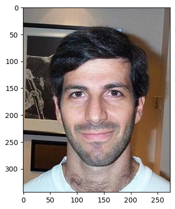
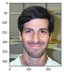
sample_idx = 539
sample = train_dataset[sample_idx]
data = sample[0]
label = sample[1]

print("Data type: {}".format(data.dtype))
print("Label: {}".format(label))
print("Label description: {}".format(train_dataset.synsets[label]))
assert label == 1

imshow(data.asnumpy(), cmap='gray')

Data type: uint8
Label: 1
Label description: Faces_easy

<matplotlib.image.AxesImage at 0x7f249bfe9550>

Using your own data with custom Datasets

Sometimes you have data that doesn’t quite fit the format expected by the included Datasets. You might be able to preprocess your data to fit the expected format, but it is easy to create your own dataset to do this.

All you need to do is create a class that implements a __getitem__ method, that returns a sample (i.e. a tuple of mx.np.ndarrays).

New in MXNet 2.0: faster C++ backend dataloaders

As part of an effort to speed up the current data loading pipeline using gluon dataset and dataloader, a new dataloader was created that uses only a C++ backend and avoids potentially slow calls to Python functions.

See original issue, pull request and implementation.

The current data loading pipeline is the major bottleneck for many training tasks. The flow can be summarized as:

• Dataset.__getitem__

• Transform.__call__()/forward()

• Batchify

• (optional communicate through shared_mem)

• split_and_load(devices)

• training on GPUs

Performance concerns include slow python dataset/transform functions, multithreading issues due to global interpreter lock, Python multiprocessing issues due to speed, and batchify issues due to poor memory management.

This new dataloader provides: - common C++ batchify functions that are split and context aware - a C++ MultithreadingDataLoader which inherit the same arguments as gluon.data.DataLoader but use MXNet internal multithreading rather than python multiprocessing. - fallback to python multiprocessing whenever the dataset is not fully supported by backend (e.g., there are custom python datasets) in the case that: - the transform is not fully hybridizable - batchify is not fully supported by backend

Users can continue to with the traditional gluon.data.Dataloader and the C++ backend will be applied automatically. The ‘try_nopython’ default is ‘Auto’, which detects whether the C++ backend is available given the dataset and transforms.

Here you will show a performance increase on a t3.2xl instance for the CIFAR10 dataset with the C++ backend.

Using the C++ backend:

cpp_dl = mx.gluon.data.DataLoader(
    mx.gluon.data.vision.CIFAR10(train=True, transform=None), batch_size=32, num_workers=2,try_nopython=True)

Downloading /home/jenkins_slave/.mxnet/datasets/cifar10/cifar-10-binary.tar.gz from https://apache-mxnet.s3-accelerate.dualstack.amazonaws.com/gluon/dataset/cifar10/cifar-10-binary.tar.gz...

start = time.time()
for _ in range(3):
    print(len(cpp_dl))
    for _ in cpp_dl:
        pass
print('Elapsed time for backend dataloader:', time.time() - start)

1563
1563
1563
Elapsed time for backend dataloader: 7.367106676101685

Using the Python backend:

dl = mx.gluon.data.DataLoader(
    mx.gluon.data.vision.CIFAR10(train=True, transform=None), batch_size=32, num_workers=2,try_nopython=False)

start = time.time()
for _ in range(3):
    print(len(dl))
    for _ in dl:
        pass
print('Elapsed time for python dataloader:', time.time() - start)

1563
1563
1563
Elapsed time for python dataloader: 8.722143650054932

Next Steps

Now that you have some experience with MXNet’s datasets and dataloaders, it’s time to use them for Step 6: Training a Neural Network.

---

Did this page help you?

Yes

No

Thanks for your feedback!

---