Normalization Blocks

When training deep neural networks there are a number of techniques that are thought to be essential for model convergence. One important area is deciding how to initialize the parameters of the network. Using techniques such as Xavier initialization, we can can improve the gradient flow through the network at the start of training. Another important technique is normalization: i.e. scaling and shifting certain values towards a distribution with a mean of 0 (i.e. zero-centered) and a standard distribution of 1 (i.e. unit variance). Which values you normalize depends on the exact method used as we’ll see later on.

Figure 1: Data Normalization (Source)

Why does this help? Some research has found that networks with normalization have a loss function that’s easier to optimize using stochastic gradient descent. Other reasons are that it prevents saturation of activations and prevents certain features from dominating due to differences in scale.

Data Normalization

One of the first applications of normalization is on the input data to the network. You can do this with the following steps:

• Step 1 is to calculate the mean and standard deviation of the entire training dataset. You’ll usually want to do this for each channel separately. Sometimes you’ll see normalization on images applied per pixel, but per channel is more common.

• Step 2 is to use these statistics to normalize each batch for training and for inference too.

Tip: A BatchNorm layer at the start of your network can have a similar effect (see ‘Beta and Gamma’ section for details on how this can be achieved). You won’t need to manually calculate and keep track of the normalization statistics.

Warning: You should calculate the normalization means and standard deviations using the training dataset only. Any leakage of information from you testing dataset will effect the reliability of your testing metrics.

When using pre-trained models from the Gluon Model Zoo you’ll usually see the normalization statistics used for training (i.e. statistics from step 1). You’ll want to use these statistics to normalize your own input data for fine-tuning or inference with these models. Using transforms.Normalize is one way of applying the normalization, and this should be used in the Dataset.

import mxnet as mx
from mxnet.gluon.data.vision.transforms import Normalize

image_int = mx.np.random.randint(low=0, high=256, size=(1,3,2,2))
image_float = image_int.astype('float32')/255
# the following normalization statistics are taken from gluon model zoo
normalizer = Normalize(mean=[0.485, 0.456, 0.406], std=[0.229, 0.224, 0.225])
image = normalizer(image_float)
image

[04:51:12] /work/mxnet/src/storage/storage.cc:202: Using Pooled (Naive) StorageManager for CPU

array([[[[-2.1007793 ,  0.57068247],
         [-1.8267832 ,  0.3651854 ]],

        [[ 0.55532223,  0.90546227],
         [-1.5630252 , -0.14495796]],

        [[ 2.4831376 , -1.4732897 ],
         [ 0.49620935,  1.3502399 ]]]])

Activation Normalization

We don’t have to limit ourselves to normalizing the inputs to the network either. A similar idea can be applied inside the network too, and we can normalize activations between certain layer operations. With deep neural networks most of the convergence benefits described are from this type of normalization.

MXNet Gluon has 3 of the most commonly used normalization blocks: BatchNorm, LayerNorm and InstanceNorm. You can use them in networks just like any other MXNet Gluon Block, and are often used after Activation Blocks.

Watch Out: Check the architecture of models carefully because sometimes the normalization is applied before the Activation.

Advanced: all of the following methods begin by normalizing certain input distribution (i.e. zero-centered with unit variance), but then shift by (a trainable parameter) beta and scale by (a trainable parameter) gamma. Overall the effect is changing the input distribution to have a mean of beta and a variance of gamma, also allowing to the network to ‘undo’ the effect of the normalization if necessary.

Batch Normalization

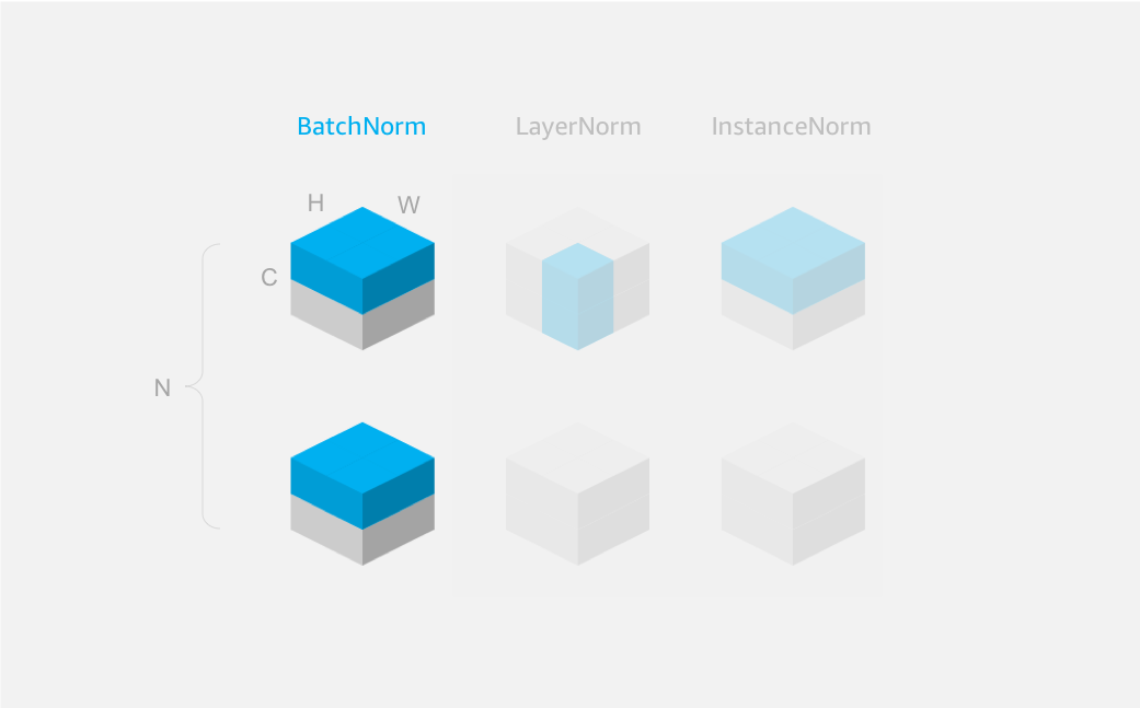
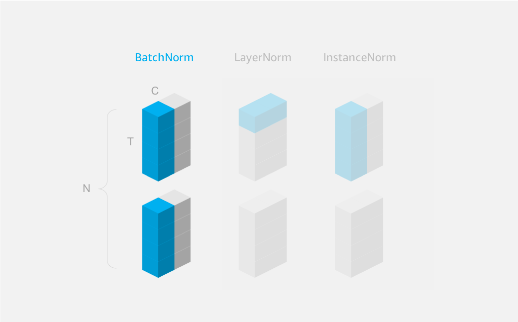
Figure 1: BatchNorm on NCHW data	Figure 2: BatchNorm on NTC data
(e.g. batch of images) using the default of axis=1	(e.g. batch of sequences) overriding the default with axis=2 (or axis=-1)

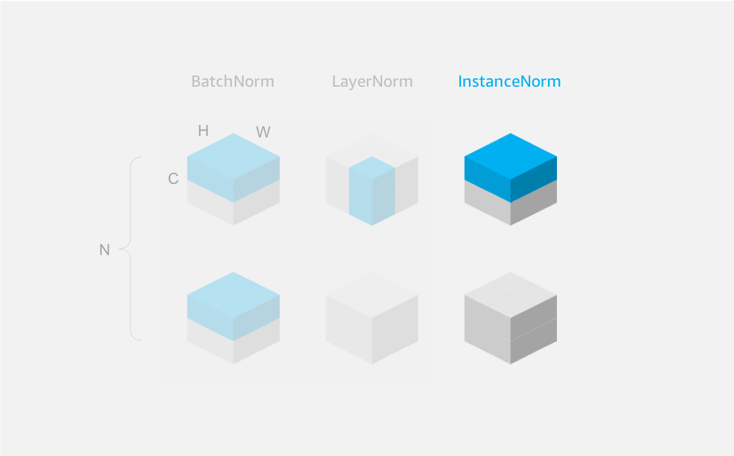
One of the most popular normalization techniques is Batch Normalization, usually called BatchNorm for short. We normalize the activations across all samples in a batch for each of the channels independently. See Figure 1. We calculate two batch (or local) statistics for every channel to perform the normalization: the mean and variance of the activations in that channel for all samples in a batch. And we use these to shift and scale respectively.

Tip: we can use this at the start of a network to perform data normalization, although this is not exactly equivalent to the data normalization example seen above (that had fixed normalization statistics). With BatchNorm the normalization statistics depend on the batch, so could change each batch, and there can also be a post-normalization shift and scale.

Warning: the estimates for the batch mean and variance can themselves have high variance when the batch size is small (or when the spatial dimensions of samples are small). This can lead to instability during training, and unreliable estimates for the global statistics.

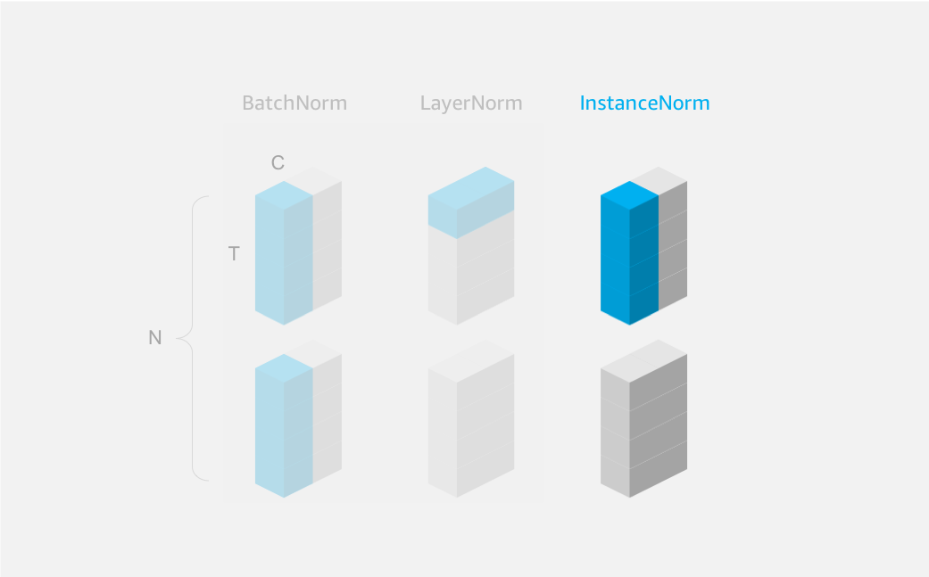
Warning: it seems that BatchNorm is better suited to convolutional networks (CNNs) than recurrent networks (RNNs). We expect the input distribution to the recurrent cell to change over time, so normalization over time doesn’t work well. LayerNorm is better suited for this case. When you do need to use BatchNorm on sequential data, make sure the axis parameter is set correctly. With data in NTC format you should set axis=2 (or axis=-1 equivalently). See Figure 2.

As an example, we’ll apply BatchNorm to a batch of 2 samples, each with 2 channels, and both height and width of 2 (in NCHW format).

data = mx.np.arange(start=0, stop=2*2*2*2).reshape(2, 2, 2, 2)
print(data)

[[[[ 0.  1.]
   [ 2.  3.]]

  [[ 4.  5.]
   [ 6.  7.]]]


 [[[ 8.  9.]
   [10. 11.]]

  [[12. 13.]
   [14. 15.]]]]

With MXNet Gluon we can apply batch normalization with the mx.gluon.nn.BatchNorm block. It can be created and used just like any other MXNet Gluon block (such as Conv2D). Its input will typically be unnormalized activations from the previous layer, and the output will be the normalized activations ready for the next layer. Since we’re using data in NCHW format we can use the default axis.

net = mx.gluon.nn.BatchNorm()

We still need to initialize the block because it has a number of trainable parameters, as we’ll see later on.

net.initialize()

We can now run the network as we would during training (under autograd.record context scope).

Remember: BatchNorm runs differently during training and inference. When training, the batch statistics are used for normalization. During inference, a exponentially smoothed average of the batch statistics that have been observed during training is used instead.

Warning: BatchNorm assumes the channel dimension is the 2nd in order (i.e. axis=1). You need to ensure your data has a channel dimension, and change the axis parameter of BatchNorm if it’s not the 2nd dimension. A batch of greyscale images of shape (100,32,32) would not work, since the 2nd dimension is height and not channel. You’d need to add a channel dimension using data.expand_dims(1) in this case to give shape (100,1,32,32).

with mx.autograd.record():
    output = net(data)
    loss = mx.np.abs(output)
loss.backward()
print(output)

[[[[-1.324244   -1.0834724 ]
   [-0.8427007  -0.60192907]]

  [[-1.324244   -1.0834724 ]
   [-0.8427007  -0.60192907]]]


 [[[ 0.60192907  0.8427007 ]
   [ 1.0834724   1.324244  ]]

  [[ 0.60192907  0.8427007 ]
   [ 1.0834724   1.324244  ]]]]

We can immediately see the activations have been scaled down and centered around zero. Activations are the same for each channel, because each channel was normalized independently. We can do a quick sanity check on these results, by manually calculating the batch mean and variance for each channel.

axes = list(range(data.ndim))
del axes[1]
batch_means = mx.np.mean(data, axis=axes)
batch_square = mx.np.square(data - batch_means.reshape(1, -1, 1, 1))
axes = list(range(batch_square.ndim))
del axes[1]
batch_vars = mx.np.mean(batch_square, axis=axes)
print('batch_means:', batch_means.asnumpy())
print('batch_vars:', batch_vars.asnumpy())

batch_means: [5.5 9.5]
batch_vars: [17.25 17.25]

And use these to scale the first entry in data, to confirm the BatchNorm calculation of -1.324 was correct.

print("manually calculated:", ((data[0][0][0][0] - batch_means[0])/mx.np.sqrt(batch_vars[0])).asnumpy())
print("automatically calculated:", output[0][0][0][0].asnumpy())

manually calculated: -1.3242445
automatically calculated: -1.324244

As mentioned before, BatchNorm has a number of parameters that update throughout training. 2 of the parameters are not updated in the typical fashion (using gradients), but instead are updated deterministically using exponential smoothing. We need to keep track of the average mean and variance of batches during training, so that we can use these values for normalization during inference.

Why are global statistics needed? Often during inference, we have a batch size of 1 so batch variance would be impossible to calculate. We can just use global statistics instead. And we might get a data distribution shift between training and inference data, which shouldn’t just be normalized away.

Advanced: when using a pre-trained model inside another model (e.g. a pre-trained ResNet as a image feature extractor inside an instance segmentation model) you might want to use global statistics of the pre-trained model during training. Setting use_global_stats=True is a method of using the global running statistics during training, and preventing the global statistics from updating. It has no effect on inference mode.

After a single step (specifically after the backward call) we can see the running_mean and running_var have been updated.

print('running_mean:', net.running_mean.data().asnumpy())
print('running_var:', net.running_var.data().asnumpy())

running_mean: [0.55000013 0.9500002 ]
running_var: [2.6250005 2.6250005]

You should notice though that these running statistics do not match the batch statistics we just calculated. And instead they are just 10% of the value we’d expect. We see this because of the exponential average process, and because the momentum parameter of BatchNorm is equal to 0.9 : i.e. 10% of the new value, 90% of the old value (which was initialized to 0). Over time the running statistics will converge to the statistics of the input distribution, while still being flexible enough to adjust to shifts in the input distribution. Using the same batch another 100 times (which wouldn’t happen in practice), we can see the running statistics converge to the batch statsitics calculated before.

for i in range(100):
    with mx.autograd.record():
        output = net(data)
        loss = mx.np.abs(output)
    loss.backward()
print('running_means:', net.running_mean.data().asnumpy())
print('running_vars:', net.running_var.data().asnumpy())

running_means: [5.49987  9.499768]
running_vars: [17.249609 17.249609]

Beta and Gamma

As mentioned previously, there are two additional parameters in BatchNorm which are trainable in the typical fashion (with gradients). beta is used to shift and gamma is used to scale the normalized distribution, which allows the network to ‘undo’ the effects of normalization if required.

Advanced: Sometimes used for input normalization, you can prevent beta shifting and gamma scaling by setting the learning rate multipler (i.e. lr_mult) of these parameters to 0. Zero centering and scaling to unit variance will still occur, only post normalization shifting and scaling will prevented. See this discussion post for details.

We haven’t updated these parameters yet, so they should still be as initialized. You can see the default for beta is 0 (i.e. not shift) and gamma is 1 (i.e. not scale), so the initial behaviour is to keep the distribution unit normalized.

print('beta:', net.beta.data().asnumpy())
print('gamma:', net.gamma.data().asnumpy())

beta: [0. 0.]
gamma: [1. 1.]

We can also check the gradient on these parameters. Since we were finding the gradient of the sum of absolute values, we would expect the gradient of gamma to be equal to the number of points in the data (i.e. 16). So to minimize the loss we’d decrease the value of gamma, which would happen as part of a trainer.step.

print('beta gradient:', net.beta.grad().asnumpy())
print('gamma gradient:', net.gamma.grad().asnumpy())

beta gradient: [0. 0.]
gamma gradient: [7.7046924 7.7046924]

Inference Mode

When it comes to inference, BatchNorm uses the global statistics that were calculated during training. Since we’re using the same batch of data over and over again (and our global running statistics have converged), we get a very similar result to using training mode. beta and gamma are also applied by default (unless explicitly removed).

output = net(data)
print(output)

[[[[-1.3242277  -1.0834533 ]
   [-0.8426789  -0.6019046 ]]

  [[-1.3242033  -1.0834289 ]
   [-0.84265447 -0.60188013]]]


 [[[ 0.6019673   0.8427416 ]
   [ 1.083516    1.3242904 ]]

  [[ 0.6019917   0.84276605]
   [ 1.0835404   1.3243148 ]]]]

Layer Normalization

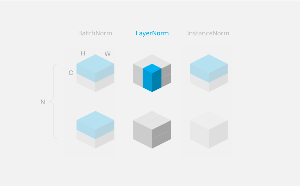
An alternative to BatchNorm that is better suited to recurrent networks (RNNs) is called LayerNorm. Unlike BatchNorm which normalizes across all samples of a batch per channel, LayerNorm normalizes across all channels of a single sample.

Some of the disadvantages of BatchNorm no longer apply. Small batch sizes are no longer an issue, since normalization statistics are calculated on single samples. And confusion around training and inference modes disappears because LayerNorm is the same for both modes.

Warning: similar to having a small batch sizes in BatchNorm, you may have issues with LayerNorm if the input channel size is small. Using embeddings with a large enough dimension size avoids this (approx >20).

Warning: currently MXNet Gluon’s implementation of LayerNorm is applied along a single axis (which should be the channel axis). Other frameworks have the option to apply normalization across multiple axes, which leads to differences in LayerNorm on NCHW input by default. See Figure 3. Other frameworks can normalize over C, H and W, not just C as with MXNet Gluon.

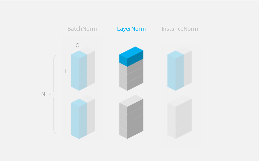
Remember: LayerNorm is intended to be used with data in NTC format so the default normalization axis is set to -1 (corresponding to C for channel). Change this to axis=1 if you need to apply LayerNorm to data in NCHW format.

Figure 3: LayerNorm on NCHW data	Figure 4: LayerNorm on NTC data
(e.g. batch of images) overriding the default with axis=1	(e.g. batch of sequences) using the default of axis=-1

As an example, we’ll apply LayerNorm to a batch of 2 samples, each with 4 time steps and 2 channels (in NTC format).

data = mx.np.arange(start=0, stop=2*4*2).reshape(2, 4, 2)
print(data)

[[[ 0.  1.]
  [ 2.  3.]
  [ 4.  5.]
  [ 6.  7.]]

 [[ 8.  9.]
  [10. 11.]
  [12. 13.]
  [14. 15.]]]

With MXNet Gluon we can apply layer normalization with the mx.gluon.nn.LayerNorm block. We need to call initialize because LayerNorm has two learnable parameters by default: beta and gamma that are used for post normalization shifting and scaling of each channel.

net = mx.gluon.nn.LayerNorm()
net.initialize()
output = net(data)
print(output)

[[[-0.99998  0.99998]
  [-0.99998  0.99998]
  [-0.99998  0.99998]
  [-0.99998  0.99998]]

 [[-0.99998  0.99998]
  [-0.99998  0.99998]
  [-0.99998  0.99998]
  [-0.99998  0.99998]]]

We can see that normalization has been applied across all channels for each time step and each sample.

We can also check the parameters beta and gamma and see that they are per channel (i.e. 2 of each in this example).

print('beta:', net.beta.data().asnumpy())
print('gamma:', net.gamma.data().asnumpy())

beta: [0. 0.]
gamma: [1. 1.]

Instance Normalization

Another less common normalization technique is called InstanceNorm, which can be useful for certain tasks such as image stylization. Unlike BatchNorm which normalizes across all samples of a batch per channel, InstanceNorm normalizes across all spatial dimensions per channel per sample (i.e. each sample of a batch is normalized independently).

Watch out: InstanceNorm is better suited to convolutional networks (CNNs) than recurrent networks (RNNs). We expect the input distribution to the recurrent cell to change over time, so normalization over time doesn’t work well. LayerNorm is better suited for this case.

Figure 3: InstanceNorm on NCHW data	Figure 4: InstanceNorm on NTC data
(e.g. batch of images) using the default axis=1	(e.g. batch of sequences) overiding the default with axis=2 (or axis=-1 equivalently)

As an example, we’ll apply InstanceNorm to a batch of 2 samples, each with 2 channels, and both height and width of 2 (in NCHW format).

data = mx.np.arange(start=0, stop=2*2*2*2).reshape(2, 2, 2, 2)
print(data)

[[[[ 0.  1.]
   [ 2.  3.]]

  [[ 4.  5.]
   [ 6.  7.]]]


 [[[ 8.  9.]
   [10. 11.]]

  [[12. 13.]
   [14. 15.]]]]

With MXNet Gluon we can apply instance normalization with the mx.gluon.nn.InstanceNorm block. We need to call initialize because InstanceNorm has two learnable parameters by default: beta and gamma that are used for post normalization shifting and scaling of each channel.

net = mx.gluon.nn.InstanceNorm()
net.initialize()
output = net(data)
print(output)

[[[[-1.3416355  -0.44721183]
   [ 0.44721183  1.3416355 ]]

  [[-1.3416355  -0.44721183]
   [ 0.44721183  1.3416355 ]]]


 [[[-1.3416355  -0.44721183]
   [ 0.44721183  1.3416355 ]]

  [[-1.3416355  -0.44721183]
   [ 0.44721183  1.3416355 ]]]]

We can also check the parameters beta and gamma and see that they are per channel (i.e. 2 of each in this example).

print('beta:', net.beta.data().asnumpy())
print('gamma:', net.gamma.data().asnumpy())

beta: [0. 0.]
gamma: [1. 1.]

---

Did this page help you?

Yes

No

Thanks for your feedback!

---