Custom Loss Blocks

All neural networks need a loss function for training. A loss function is a quantitive measure of how bad the predictions of the network are when compared to ground truth labels. Given this score, a network can improve by iteratively updating its weights to minimise this loss. Some tasks use a combination of multiple loss functions, but often you’ll just use one. MXNet Gluon provides a number of the most commonly used loss functions, and you’ll choose certain functions depending on your network and task. Some common task and loss function pairs include:

• Regression: L1Loss, L2Loss

• Classification: SigmoidBinaryCrossEntropyLoss, SoftmaxCrossEntropyLoss

• Embeddings: HingeLoss

However, we may sometimes want to solve problems that require customized loss functions; this tutorial shows how we can do that in Gluon. We will implement contrastive loss which is typically used in Siamese networks.

import matplotlib.pyplot as plt
import mxnet as mx
from mxnet import autograd, gluon, np, npx
from mxnet.gluon.loss import Loss
import random

What is Contrastive Loss

Contrastive loss is a distance-based loss function. During training, pairs of images are fed into a model. If the images are similar, the loss function will return 0, otherwise 1.

Y is a binary label indicating similarity between training images. Contrastive loss uses the Euclidean distance D between images and is the sum of 2 terms: - the loss for a pair of similar points - the loss for a pair of dissimilar points

The loss function uses a margin m which is has the effect that dissimlar pairs only contribute if their loss is within a certain margin.

In order to implement such a customized loss function in Gluon, we just need to define a new class that is inheriting from the Loss base class. We then define the contrastive loss logic in the forward method. This method takes the images image1, image2 and the label which defines whether image1 and image2 are similar (=0) or dissimilar (=1). Gluon’s Loss base class is in fact a HybridBlock, and we hybridize our custom loss function, we can get performance speedups.

class ContrastiveLoss(Loss):
    def __init__(self, margin=6., weight=None, batch_axis=0, **kwargs):
        super(ContrastiveLoss, self).__init__(weight, batch_axis, **kwargs)
        self.margin = margin

    def forward(self, image1, image2, label):
        distances = image1 - image2
        distances_squared = np.sum(np.square(distances), 1, keepdims=True)
        euclidean_distances = np.sqrt(distances_squared + 0.0001)
        d = np.clip(self.margin - euclidean_distances, 0, self.margin)
        loss = (1 - label) * distances_squared + label * np.square(d)
        loss = 0.5*loss
        return loss
loss = ContrastiveLoss(margin=6.0)

Define the Siamese network

A Siamese network consists of 2 identical networks, that share the same weights. They are trained on pairs of images and each network processes one image. The label defines whether the pair of images is similar or not. The Siamese network learns to differentiate between two input images.

Our network consists of 2 convolutional and max pooling layers that downsample the input image. The output is then fed through a fully connected layer with 256 hidden units and another fully connected layer with 2 hidden units.

class Siamese(gluon.HybridBlock):
    def __init__(self, **kwargs):
        super(Siamese, self).__init__(**kwargs)
        self.cnn = gluon.nn.HybridSequential()
        self.cnn.add(gluon.nn.Conv2D(64, 5, activation='relu'))
        self.cnn.add(gluon.nn.MaxPool2D(2, 2))
        self.cnn.add(gluon.nn.Conv2D(64, 5, activation='relu'))
        self.cnn.add(gluon.nn.MaxPool2D(2, 2))
        self.cnn.add(gluon.nn.Dense(256, activation='relu'))
        self.cnn.add(gluon.nn.Dense(2, activation='softrelu'))

    def forward(self, input0, input1):
        out0 = self.cnn(input0)
        out1 = self.cnn(input1)
        return out0, out1

Prepare the training data

We train our network on the Ominglot dataset which is a collection of 1623 hand drawn characters from 50 alphabets. You can download it from here. We need to create a dataset that contains a random set of similar and dissimilar images. We use Gluon’s ImageFolderDataset where we overwrite __getitem__ and randomly return similar and dissimilar pairs of images.

class GetImagePairs(mx.gluon.data.vision.ImageFolderDataset):
    def __init__(self, root):
        super(GetImagePairs, self).__init__(root, flag=0)
        self.root = root

    def __getitem__(self, index):
        items_with_index = list(enumerate(self.items))
        image0_index, image0_tuple = random.choice(items_with_index)
        should_get_same_class = random.randint(0, 1)
        if should_get_same_class:
            while True:
                image1_index, image1_tuple = random.choice(items_with_index)
                if image0_tuple[1] == image1_tuple[1]:
                    break
        else:
            image1_index, image1_tuple = random.choice(items_with_index)
        image0 = super().__getitem__(image0_index)
        image1 = super().__getitem__(image1_index)
        label = mx.np.array([int(image1_tuple[1] != image0_tuple[1])])
        return image0[0], image1[0], label

    def __len__(self):
        return super().__len__()

We train the network on a subset of the data, the Tifinagh alphabet. Once the model is trained we test it on the Inuktitut alphabet.

def transform(img0, img1, label):
    normalized_img0 = nd.transpose(img0.astype('float32'), (2, 0, 1))/255.0
    normalized_img1 = nd.transpose(img1.astype('float32'), (2, 0, 1))/255.0
    return normalized_img0, normalized_img1, label

training_dir = "images_background/Tifinagh"
testing_dir = "images_background/Inuktitut_(Canadian_Aboriginal_Syllabics)"
train = GetImagePairs(training_dir)
test = GetImagePairs(testing_dir)
train_dataloader = gluon.data.DataLoader(train.transform(transform),
                                        shuffle=True, batch_size=16)
test_dataloader = gluon.data.DataLoader(test.transform(transform),
                                        shuffle=False, batch_size=1)

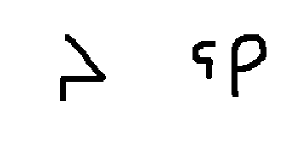
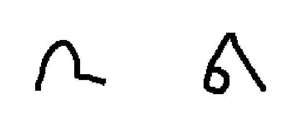
Following code plots some examples from the test dataset.

img1, img2, label = test[0]
print("Same: {}".format(int(label.item()) == 0))
fig, (ax0, ax1) = plt.subplots(ncols=2, figsize=(10, 5))
ax0.imshow(img1.asnumpy()[:,:,0], cmap='gray')
ax0.axis('off')
ax1.imshow(img2.asnumpy()[:,:,0], cmap='gray')
ax1.axis("off")
plt.show()

Train the Siamese network

Before we can start training, we need to instantiate the custom constrastive loss function and initialize the model.

model = Siamese()
model.initialize(init=mx.init.Xavier())
trainer = gluon.Trainer(model.collect_params(), 'adam', {'learning_rate': 0.001})
loss = ContrastiveLoss(margin=6.0)

Start the training loop:

for epoch in range(10):
    for i, data in enumerate(train_dataloader):
        image1, image2, label = data
        with autograd.record():
            output1, output2 = model(image1, image2)
            loss_contrastive = loss(output1, output2, label)
        loss_contrastive.backward()
        trainer.step(image1.shape[0])
        loss_mean = loss_contrastive.mean().item()
        print("Epoch number {}\n Current loss {}\n".format(epoch, loss_mean))

Test the trained Siamese network

During inference we compute the Euclidean distance between the output vectors of the Siamese network. High distance indicates dissimilarity, low values indicate similarity.

for i, data in enumerate(test_dataloader):
    img1, img2, label = data
    output1, output2 = model(img1, img2)
    dist_sq = mx.np.sum(mx.np.square(output1 - output2))
    dist = mx.np.sqrt(dist_sq).item()
    print("Euclidean Distance:", dist, "Test label", label[0].item())
    fig, (ax0, ax1) = plt.subplots(ncols=2, figsize=(10, 5))
    ax0.imshow(img1.asnumpy()[0, 0, :, :], cmap='gray')
    ax0.axis('off')
    ax1.imshow(img2.asnumpy()[0, 0, :, :], cmap='gray')
    ax1.axis("off")
    plt.show()

Common pitfalls with custom loss functions

When customizing loss functions, we may encounter certain pitfalls. If the loss is not decreasing as expected or if forward/backward pass is crashing, then one should check the following:

Activation function in the last layer

Verify whether the last network layer uses the correct activation function: for instance in binary classification tasks we need to apply a sigmoid on the output data. If we use this activation in the last layer and define a loss function like Gluon’s SigmoidBinaryCrossEntropy, we would basically apply sigmoid twice and the loss would not converge as expected. If we don’t define any activation function, Gluon will per default apply a linear activation.

Intermediate loss values

In our example, we computed the square root of squared distances between 2 images: F.sqrt(distances_squared). If images are very similar we take the sqare root of a value close to 0, which can lead to NaN values. Adding a small epsilon to distances_squared avoids this problem.

Shape of intermediate loss vectors

In most cases having the wrong tensor shape will lead to an error, as soon as we compare data with labels. But in some cases, we may be able to normally run the training, but it does not converge. For instance, if we don’t set keepdims=True in our customized loss function, the shape of the tensor changes. The example still runs fine but does not converge.

If you encounter a similar problem, then it is useful to check the tensor shape after each computation step in the loss function.

Differentiable

Backprogration requires the loss function to be differentiable. If the customized loss function cannot be differentiated the backward pass will crash.

---

Did this page help you?

Yes

No

Thanks for your feedback!

---